本文介绍了使用Paddle实现神经网络热力图(CAM)可视化的方法。CAM可展示CNN分类时关注的区域,文中详细阐述其原理,提供了完整代码,包括图像预处理、模型输出提取、梯度计算等步骤,还说明如何通过热力图指导数据集扩充和数据增强,帮助优化模型性能。
☞☞☞AI 智能聊天, 问答助手, AI 智能搜索, 免费无限量使用 DeepSeek R1 模型☜☜☜

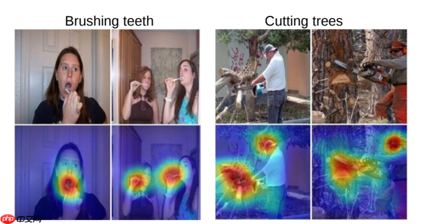
Class Activation Mapping(CAM)是一个帮助可视化CNN的工具,通过它我们可以观察为了达到正确分类的目的,网络更侧重于哪块区域。比如,下面两幅图,一个是刷牙,一个是砍树,我们根据热力图可以看到高响应区域的确集中在我们认为最有助于作出判断的部位。
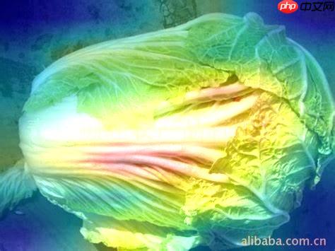
本项目最初还是来自于项目:讯飞农作物生长情况识别挑战赛baseline(非官方),因为数据集不大,尽管模型收敛很好,但线上的分数确始终不能更进一步。于是想到可以可视化一下网络的CAM,观察一下指导分类的高响应区域是否落在目标核心部位上。
CAM论文链接地址
!cd 'data/data106772' && unzip -q img.zip
%matplotlib inlineimport osfrom PIL import Imageimport paddleimport numpy as npimport cv2import matplotlib.pyplot as pltfrom draw_features import Res2Net_vdimport paddle.nn.functional as Fimport paddleimport warnings
warnings.filterwarnings('ignore')def draw_CAM(model, img_path, save_path, transform=None, visual_heatmap=False):
    '''
    绘制 Class Activation Map
    :param model: 加载好权重的Pytorch model
    :param img_path: 测试图片路径
    :param save_path: CAM结果保存路径
    :param transform: 输入图像预处理方法
    :param visual_heatmap: 是否可视化原始heatmap(调用matplotlib)
    :return:
    '''
    # 图像加载&预处理
    img = Image.open(img_path).convert('RGB')
    img = img.resize((224, 224), Image.BILINEAR) #Image.BILINEAR双线性插值
    if transform:
        img = transform(img)    # img = img.unsqueeze(0)
    img = np.array(img).astype('float32')
    img = img.transpose((2, 0, 1))
    img = paddle.to_tensor(img)
    img = paddle.unsqueeze(img, axis=0)    # print(img.shape)
    # 获取模型输出的feature/score

    output,features = model(img)    print('outputshape:',output.shape)    print('featureshape:',features.shape)    # lab = np.argmax(out.numpy())
    # 为了能读取到中间梯度定义的辅助函数
    def extract(g):
        global features_grad
        features_grad = g
    # 预测得分最高的那一类对应的输出score
    pred = np.argmax(output.numpy())    # print('***********pred:',pred)
    pred_class = output[:, pred]    # print(pred_class)

    features.register_hook(extract)
    pred_class.backward() # 计算梯度

    grads = features_grad   # 获取梯度
    # print(grads.shape)
    # pooled_grads = paddle.nn.functional.adaptive_avg_pool2d( x = grads, output_size=[1, 1])
    pooled_grads = grads
    # 此处batch size默认为1,所以去掉了第0维(batch size维)
    pooled_grads = pooled_grads[0]    # print('pooled_grads:', pooled_grads.shape)
    # print(pooled_grads.shape)
    features = features[0]    # print(features.shape)
    # 最后一层feature的通道数
    for i in range(2048):
        features[i, ...] *= pooled_grads[i, ...]

    heatmap = features.detach().numpy()

    heatmap = np.mean(heatmap, axis=0)    # print(heatmap)
    heatmap = np.maximum(heatmap, 0)    # print('+++++++++',heatmap)
    heatmap /= np.max(heatmap)    # print('+++++++++',heatmap)
    # 可视化原始热力图
    if visual_heatmap:
        plt.matshow(heatmap)
        plt.show()

    img = cv2.imread(img_path)  # 用cv2加载原始图像
    heatmap = cv2.resize(heatmap, (img.shape[1], img.shape[0]))  # 将热力图的大小调整为与原始图像相同
    heatmap = np.uint8(255 * heatmap)  # 将热力图转换为RGB格式
    # print(heatmap.shape)
    heatmap = cv2.applyColorMap(heatmap, cv2.COLORMAP_JET)  # 将热力图应用于原始图像
    superimposed_img = heatmap * 0.4 + img  # 这里的0.4是热力图强度因子
    cv2.imwrite(save_path, superimposed_img)  # 将图像保存到硬盘model_re2 = Res2Net_vd(layers=50, scales=4, width=26, class_dim=4)# model_re2 = Res2Net50_vd_26w_4s(class_dim=4)modelre2_state_dict = paddle.load("Hapi_MyCNN.pdparams")
model_re2.set_state_dict(modelre2_state_dict, use_structured_name=True)
use_gpu = Truepaddle.set_device('gpu:0') if use_gpu else paddle.set_device('cpu')

model_re2.eval()

draw_CAM(model_re2, 'data/data106772/img/test/629.jpg', 'test3.jpg', transform=None, visual_heatmap=True)W1123 17:02:34.611114 6534 device_context.cc:447] Please NOTE: device: 0, GPU Compute Capability: 7.0, Driver API Version: 10.1, Runtime API Version: 10.1 W1123 17:02:34.615968 6534 device_context.cc:465] device: 0, cuDNN Version: 7.6.
outputshape: [1, 4]
featureshape: [1, 2048, 7, 7]
<Figure size 288x288 with 1 Axes>
关于代码,相信注释已经写得很明白了,需要注意的是,我把网络结构多返回了softmax层之前的特征向量,代码如下所示:
    def forward(self, inputs):        y = self.conv1_1(inputs)        y = self.conv1_2(y)        y = self.conv1_3(y)        y = self.pool2d_max(y)        blocks = []
        for block in self.block_list:            y = block(y)            blocks.append(y)        # draw_features(32, 32, y.cpu().numpy(), "{}/f7_layer3.png".format(savepath))
        # y = self.convf_1(y)
y = self.pool2d_avg(y) y = paddle.reshape(y, shape=[-1, self.pool2d_avg_channels]) out = self.out(y) blocks.append(out) return blocks[-1:-3:-1]通过该可视化方法,可以有针对性的对数据集进行扩充,以此来指导数据增强的方向。需要注意的是,大家需要对网络结构足够了解,CAM主要使用最后一层的特征向量,大家注意区分。
<br/>
以上就是Paddle可视化神经网络热力图(CAM)的详细内容,更多请关注php中文网其它相关文章!

每个人都需要一台速度更快、更稳定的 PC。随着时间的推移,垃圾文件、旧注册表数据和不必要的后台进程会占用资源并降低性能。幸运的是,许多工具可以让 Windows 保持平稳运行。

 广告
广告


Copyright 2014-2025 https://www.php.cn/ All Rights Reserved | php.cn | 湘ICP备2023035733号


 637
637