本文围绕第七届全国大学生工程训练综合能力竞赛“智能+”赛道生活垃圾智能分类任务,设计基于Ghost Module的分类算法。通过多途径采集数据,经处理后,分别用MobileNetV2测试,复现Ghost Module并构建Ghost-VGG-11,对比其与VGG-11性能,为垃圾分类装置提供算法支持。
☞☞☞AI 智能聊天, 问答助手, AI 智能搜索, 免费无限量使用 DeepSeek R1 模型☜☜☜

第七届全国大学生工程训练综合能力竞赛“智能+”赛道之生活垃圾智能分类解决方案
以日常生活垃圾分类为主题,自主设计并制作一 台根据给定任务完成生活垃圾智能分类的装置。该装置能够实现对投入的“可回收垃圾、厨余垃圾、有害垃圾和其他垃圾”等四类城市生活垃圾具有自主判别、分类、投放到相应的垃圾桶、满载报警、播放垃圾分类宣传片等功能。
待生活垃圾智能分类装置识别的四类垃圾主要包括:
使用英伟达的Jetson Nano以及树莓派摄像头采集数据。

以下代码请在Jetson Nano上运行:
import osimport cv2import numpy as npimport time

path = os.path.split(os.path.realpath(__file__))[0]
save_name="img"def mkdir(path):
    if not os.path.exists(path):
        os.makedirs(path)        print("----- new folder -----")    else:        print('----- there is this folder -----')def gstreamer_pipeline(
    capture_width=1280,
    capture_height=720,
    display_width=1280,
    display_height=720,
    framerate=60,
    flip_method=0,):
    return (        "nvarguscamerasrc ! "
        "video/x-raw(memory:NVMM), "
        "width=(int)%d, height=(int)%d, "
        "format=(string)NV12, framerate=(fraction)%d/1 ! "
        "nvvidconv flip-method=%d ! "
        "video/x-raw, width=(int)%d, height=(int)%d, format=(string)BGRx ! "
        "videoconvert ! "
        "video/x-raw, format=(string)BGR ! appsink"
        % (
            capture_width,
            capture_height,
            framerate,
            flip_method,
            display_width,
            display_height,
        )
    )def save_image_process():
    mkdir(path+"/garbagedata")
    mkdir(path+"/garbagedata/"+save_name)    print(gstreamer_pipeline(flip_method=0))
    cap = cv2.VideoCapture(gstreamer_pipeline(flip_method=0), cv2.CAP_GSTREAMER)    if cap.isOpened():
        window_handle = cv2.namedWindow("CSI Camera", cv2.WINDOW_AUTOSIZE)
        imgInd = 0
        # Window
        while cv2.getWindowProperty("CSI Camera", 0) >= 0:
            ret_val, img = cap.read()
            cv2.imshow("CSI Camera", img)
            cv2.imwrite(path+"/garbagedata/"+save_name+"/{}.jpg".format(imgInd), img)            print("imgInd=",imgInd)
            imgInd+=1
            time.sleep(0.5)            # This also acts as
            keyCode = cv2.waitKey(30) & 0xFF
            # Stop the program on the ESC key
            if keyCode == 27:                break
        cap.release()
        cv2.destroyAllWindows()    else:        print("Unable to open camera")if __name__ == '__main__':
save_image_process()执行界面如图所示: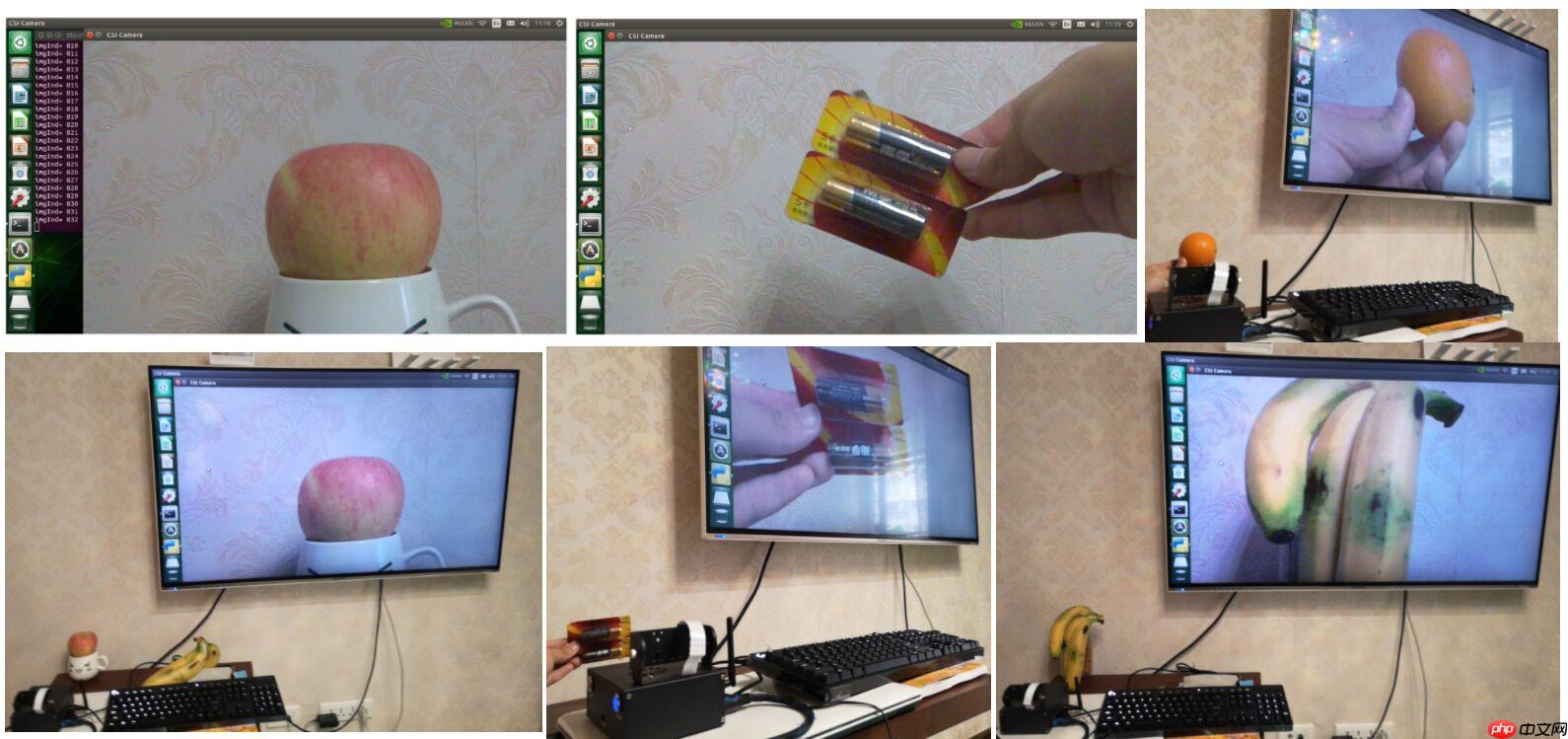
# 安装必要的库!pip install bs4
Looking in indexes: https://mirror.baidu.com/pypi/simple/
Collecting bs4
  Downloading https://mirror.baidu.com/pypi/packages/10/ed/7e8b97591f6f456174139ec089c769f89a94a1a4025fe967691de971f314/bs4-0.0.1.tar.gz
Collecting beautifulsoup4 (from bs4)
  Downloading https://mirror.baidu.com/pypi/packages/d1/41/e6495bd7d3781cee623ce23ea6ac73282a373088fcd0ddc809a047b18eae/beautifulsoup4-4.9.3-py3-none-any.whl (115kB)
     |████████████████████████████████| 122kB 11.6MB/s eta 0:00:01
Collecting soupsieve>1.2; python_version >= "3.0" (from beautifulsoup4->bs4)
  Downloading https://mirror.baidu.com/pypi/packages/02/fb/1c65691a9aeb7bd6ac2aa505b84cb8b49ac29c976411c6ab3659425e045f/soupsieve-2.1-py3-none-any.whl
Building wheels for collected packages: bs4
  Building wheel for bs4 (setup.py) ... done
  Created wheel for bs4: filename=bs4-0.0.1-cp37-none-any.whl size=1273 sha256=1772c487d510a09bde26399526ab8e320c10db8c3c0b75caf5268c67fc816829
  Stored in directory: /home/aistudio/.cache/pip/wheels/80/e7/37/62c60fe0c1017a55e897489ce5d5e850fa5610745d6352ed0c
Successfully built bs4
Installing collected packages: soupsieve, beautifulsoup4, bs4
Successfully installed beautifulsoup4-4.9.3 bs4-0.0.1 soupsieve-2.1# 爬虫代码,运行后根据提示输入即可import reimport requestsfrom urllib import errorfrom bs4 import BeautifulSoup
import os
num = 0numPicture = 0file = ''List = []
def Find(url, A):
global List
print('正在检测图片总数,请稍等.....')
t = 0
i = 1
s = 0
while t < 1000:
Url = url + str(t) try: # 这里搞了下
Result = A.get(Url, timeout=7, allow_redirects=False) except BaseException:
t = t + 60
continue
else:
result = Result.text
pic_url = re.findall('"objURL":"(.*?)",', result, re.S) # 先利用正则表达式找到图片url
s += len(pic_url) if len(pic_url) == 0: break
else: List.append(pic_url)
t = t + 60
return s
def recommend(url):
Re = [] try:
html = requests.get(url, allow_redirects=False) except error.HTTPError as e: return
else:
html.encoding = 'utf-8'
bsObj = BeautifulSoup(html.text, 'html.parser')
div = bsObj.find('div', id='topRS') if div is not None:
listA = div.findAll('a') for i in listA: if i is not None:
Re.append(i.get_text()) return Re
def dowmloadPicture(html, keyword):
global num # t =0
pic_url = re.findall('"objURL":"(.*?)",', html, re.S) # 先利用正则表达式找到图片url
print('找到关键词:' + keyword + '的图片,即将开始下载图片...') for each in pic_url: print('正在下载第' + str(num + 1) + '张图片,图片地址:' + str(each)) try: if each is not None:
pic = requests.get(each, timeout=7) else: continue
except BaseException: print('错误,当前图片无法下载') continue
else:
string = file + r'/' + keyword + '_' + str(num) + '.jpg'
fp = open(string, 'wb')
fp.write(pic.content)
fp.close()
num += 1
if num >= numPicture: return
if __name__ == '__main__': # 主函数入口
headers = { 'Accept-Language': 'zh-CN,zh;q=0.8,zh-TW;q=0.7,zh-HK;q=0.5,en-US;q=0.3,en;q=0.2', 'Connection': 'keep-alive', 'User-Agent': 'Mozilla/5.0 (X11; Linux x86_64; rv:60.0) Gecko/20100101 Firefox/60.0', 'Upgrade-Insecure-Requests': '1'
}
A = requests.Session()
A.headers = headers
word = input("请输入搜索关键词(可以是人名,地名等): ") # add = 'http://image.baidu.com/search/flip?tn=baiduimage&ie=utf-8&word=%E5%BC%A0%E5%A4%A9%E7%88%B1&pn=120'
url = 'https://image.baidu.com/search/flip?tn=baiduimage&ie=utf-8&word=' + word + '&pn='
# 这里搞了下
tot = Find(url, A)
Recommend = recommend(url) # 记录相关推荐
print('经过检测%s类图片共有%d张' % (word, tot))
numPicture = int(input('请输入想要下载的图片数量 '))
file = input('请建立一个存储图片的文件夹,输入文件夹名称即可')
y = os.path.exists(file) if y == 1: print('该文件已存在,请重新输入')
file = input('请建立一个存储图片的文件夹,)输入文件夹名称即可')
os.mkdir(file) else:
os.mkdir(file)
t = 0
tmp = url while t < numPicture: try:
url = tmp + str(t)
# 这里搞了下
result = A.get(url, timeout=10, allow_redirects=False) except error.HTTPError as e: print('网络错误,请调整网络后重试')
t = t + 60
else:
dowmloadPicture(result.text, word)
t = t + 60
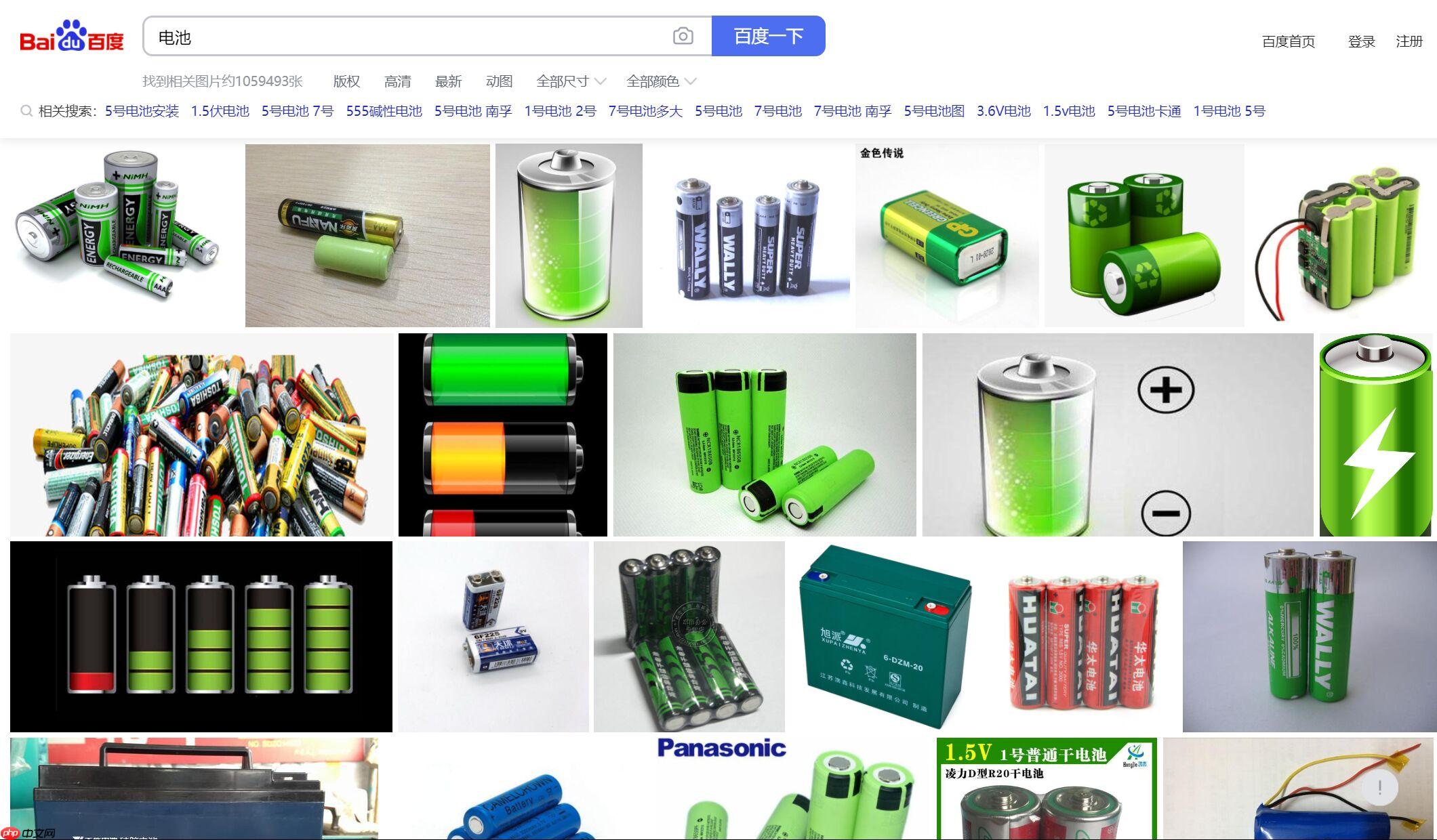
for re in Recommend: print(re, end=' ')请输入搜索关键词(可以是人名,地名等): 正在检测图片总数,请稍等..... 经过检测电池类图片共有1020张
请输入想要下载的图片数量
请建立一个存储图片的文件夹,输入文件夹名称即可找到关键词:电池的图片,即将开始下载图片...
正在下载第1张图片,图片地址:https://gimg2.baidu.com/image_search/src=http%3A%2F%2Fwww.t-chs.com%2FtuhsJDEwLmFsaWNkbi5jb20vaTIvNjQ4Mzc4ODUyL1RCMnFkd1VjQzNQTDFKalNaRnRYWGNsUlZYYV8hITY0ODM3ODg1MiQ5.jpg&refer=http%3A%2F%2Fwww.t-chs.com&app=2002&size=f9999,10000&q=a80&n=0&g=0n&fmt=jpeg?sec=1613873211&t=ee9ac8cfae2ee7a4d45e9705450f4336
正在下载第2张图片,图片地址:https://gimg2.baidu.com/image_search/src=http%3A%2F%2Fbpic.588ku.com%2Felement_origin_min_pic%2F16%2F10%2F09%2F2157fa405e95031.jpg&refer=http%3A%2F%2Fbpic.588ku.com&app=2002&size=f9999,10000&q=a80&n=0&g=0n&fmt=jpeg?sec=1613873211&t=9f70cb8588023c8ec7feff83a983cf73
正在下载第3张图片,图片地址:https://gimg2.baidu.com/image_search/src=http%3A%2F%2Fimg002.file.rongbiz.cn%2Fuploadfile%2F201307%2F27%2F03%2F47-00-78837.jpg&refer=http%3A%2F%2Fimg002.file.rongbiz.cn&app=2002&size=f9999,10000&q=a80&n=0&g=0n&fmt=jpeg?sec=1613873211&t=e68ca1e77a9001d5300055cee4a1256e
正在下载第4张图片,图片地址:https://gimg2.baidu.com/image_search/src=http%3A%2F%2Fimg.zcool.cn%2Fcommunity%2F012c8355410d64000001e71b39c9bc.jpg&refer=http%3A%2F%2Fimg.zcool.cn&app=2002&size=f9999,10000&q=a80&n=0&g=0n&fmt=jpeg?sec=1613873211&t=2988c68a74654217d4a1d656e8b8af8f
正在下载第5张图片,图片地址:https://gimg2.baidu.com/image_search/src=http%3A%2F%2Fapp.materials.cn%2Fupload%2F201508%2F25%2F201508252324292728.jpg&refer=http%3A%2F%2Fapp.materials.cn&app=2002&size=f9999,10000&q=a80&n=0&g=0n&fmt=jpeg?sec=1613873211&t=5347da7d75564c1f2c14285a9dc4b8a8
正在下载第6张图片,图片地址:https://gimg2.baidu.com/image_search/src=http%3A%2F%2Fgss0.baidu.com%2F-fo3dSag_xI4khGko9WTAnF6hhy%2Fzhidao%2Fpic%2Fitem%2Fc75c10385343fbf22c095080b27eca8065388f68.jpg&refer=http%3A%2F%2Fgss0.baidu.com&app=2002&size=f9999,10000&q=a80&n=0&g=0n&fmt=jpeg?sec=1613873211&t=70af3066ba1e81dcc4c4593d94ad4544
正在下载第7张图片,图片地址:https://gimg2.baidu.com/image_search/src=http%3A%2F%2Fa3.att.hudong.com%2F55%2F43%2F20300000926969131235438195884.jpg&refer=http%3A%2F%2Fa3.att.hudong.com&app=2002&size=f9999,10000&q=a80&n=0&g=0n&fmt=jpeg?sec=1613873211&t=66fc0d23c0668735eb561bf40ea6d792
正在下载第8张图片,图片地址:https://gimg2.baidu.com/image_search/src=http%3A%2F%2Fimg2.99114.com%2Fgroup1%2FM00%2FBD%2F2E%2FwKgGTFVDChCAa3rYAAMUd7nmdTU407.jpg&refer=http%3A%2F%2Fimg2.99114.com&app=2002&size=f9999,10000&q=a80&n=0&g=0n&fmt=jpeg?sec=1613873211&t=22a4c9ed53b9ef69d2bfae59c9b62379
正在下载第9张图片,图片地址:https://gimg2.baidu.com/image_search/src=http%3A%2F%2Fwww.t-chs.com%2FtuhsJDEwLmFsaWNkbi5jb20vaTIvMTA2NTYwODQ2L1RCMjRjWWhmYkptcHVGalNaRndYWGFFNFZYYV8hITEwNjU2MDg0NiQ5.jpg&refer=http%3A%2F%2Fwww.t-chs.com&app=2002&size=f9999,10000&q=a80&n=0&g=0n&fmt=jpeg?sec=1613873211&t=8e0da807bd4d79867901e438cd5b947c
正在下载第10张图片,图片地址:https://gimg2.baidu.com/image_search/src=http%3A%2F%2Fpic.51yuansu.com%2Fpic3%2Fcover%2F00%2F82%2F69%2F58c87a8a5e207_610.jpg&refer=http%3A%2F%2Fpic.51yuansu.com&app=2002&size=f9999,10000&q=a80&n=0&g=0n&fmt=jpeg?sec=1613873211&t=fd515ab8371594027bd108cd2602873b
数据集来源于2019华为云AI大赛·垃圾分类挑战杯,包含40个类别的垃圾图片。将40个类别进行整理:
数据集链接:https://aistudio.baidu.com/aistudio/datasetdetail/16284

数据的好坏在一定程度上决定了模型的好坏,为了提高模型的准确率,通常可以对数据集做以下处理:
为了便于PaddlePaddle加载数据集,我们需要将图片整理成数据集:
Augmentor包含许多用于标准图像处理功能的类,例如Rotate 旋转类、Crop 裁剪类等等。 包含的操作有:旋转rotate、裁剪crop、透视perspective skewing、shearing、弹性形变Elastic Distortions、亮度、对比度、颜色等等。
下面是使用Augmentor进行图像增强的参考代码:
# 安装Augmentor!pip install Augmentor
Looking in indexes: https://mirror.baidu.com/pypi/simple/
Collecting Augmentor
  Downloading https://mirror.baidu.com/pypi/packages/cb/79/861f38d5830cff631e30e33b127076bfef8ac98171e51daa06df0118c75f/Augmentor-0.2.8-py2.py3-none-any.whl
Requirement already satisfied: tqdm>=4.9.0 in /opt/conda/envs/python35-paddle120-env/lib/python3.7/site-packages (from Augmentor) (4.36.1)
Requirement already satisfied: Pillow>=5.2.0 in /opt/conda/envs/python35-paddle120-env/lib/python3.7/site-packages (from Augmentor) (7.1.2)
Requirement already satisfied: future>=0.16.0 in /opt/conda/envs/python35-paddle120-env/lib/python3.7/site-packages (from Augmentor) (0.18.0)
Requirement already satisfied: numpy>=1.11.0 in /opt/conda/envs/python35-paddle120-env/lib/python3.7/site-packages (from Augmentor) (1.16.4)
Installing collected packages: Augmentor
Successfully installed Augmentor-0.2.8
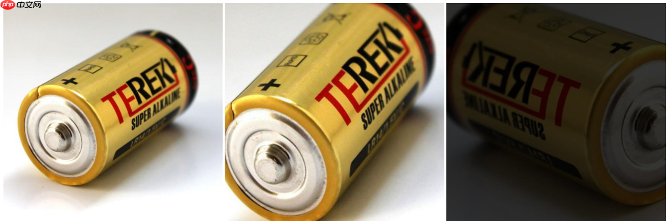
#导入数据增强工具import Augmentor
#确定原始图像存储路径以及掩码文件存储路径picture = Augmentor.Pipeline(r"battery")
#图像旋转: 按照概率0.8执行,最大左旋角度20,最大右旋角度20picture.rotate(probability=0.8, max_left_rotation=20, max_right_rotation=20)
#图像左右互换: 按照概率0.4执行picture.flip_left_right(probability=0.4)
#图像放大缩小: 按照概率0.6执行,面积为原始图0.85倍picture.zoom_random(probability=0.6, percentage_area=0.85)#图像亮度改变: 按照概率0.75执行picture.random_brightness(probability=0.75,min_factor=0.2,max_factor=0.8)
#最终扩充的数据样本数picture.sample(10)
Executing Pipeline: 0%| | 0/10 [00:00<?, ? Samples/s]
Initialised with 5 image(s) found.
Output directory set to battery/output.
Processing <PIL.Image.Image image mode=RGB size=600x600 at 0x7FBFA0593B50>: 0%| | 0/10 [00:00<?, ? Samples/s]
Processing <PIL.Image.Image image mode=RGB size=500x400 at 0x7FBFA3249F90>: 100%|██████████| 10/10 [00:02<00:00, 4.12 Samples/s]
生成前后的图片对比如下所示(左数第一张为原图,后两张为根据原图生成的图片):
图像处理工具包PIL(Python Image Library),该软件包提供了基本的图像处理功能,如:改变图像大小,旋转图像,图像格式转换,色场空间转换,图像增强,直方图处理,插值和滤波等等。
查看处理前图片的大小:
import osfrom PIL import Image# 图片文件夹路径path = "battery/output/"for filename in os.listdir(path):
img = Image.open(path + filename) print("{}的大小是{}".format(img.filename, img.size))battery/output/battery_original_电池_2.jpg_5c3e37bf-3897-4695-8a29-b3bb837a8de5.jpg的大小是(600, 600) battery/output/battery_original_电池_1.jpg_f8fc002a-eea5-4473-85b1-9bfaf1fbb170.jpg的大小是(612, 792) battery/output/battery_original_电池_2.jpg_b918f379-5dbe-4822-833b-69433950e11d.jpg的大小是(600, 600) battery/output/battery_original_电池_5.jpg_62be292d-a36d-4c78-870e-3a6fd552aee8.jpg的大小是(3264, 2448) battery/output/battery_original_电池_4.jpg_012c0cde-25a7-40e2-9873-08c233e839c7.jpg的大小是(500, 400) battery/output/battery_original_电池_1.jpg_6b99a9c9-c86d-499b-8df4-f9798a7f59dc.jpg的大小是(612, 792) battery/output/battery_original_电池_1.jpg_a353b072-fdda-4a10-be21-428d410737b5.jpg的大小是(612, 792) battery/output/battery_original_电池_7.jpg_93141dc1-2df9-4417-ae67-8788289143b4.jpg的大小是(800, 725) battery/output/battery_original_电池_1.jpg_d9e0a124-74ba-4a9a-810b-1ea2c60a6426.jpg的大小是(612, 792) battery/output/battery_original_电池_5.jpg_97906199-c600-4e6f-bc2e-2bdcaf72a84c.jpg的大小是(3264, 2448)
import osfrom PIL import Image# 图片文件夹路径path = "battery/output/"for filename in os.listdir(path):
    img = Image.open(path + filename)
    img = img.resize((1280,720),Image.ANTIALIAS) # 转换图片,图像尺寸变为1280*720
    img = img.convert('RGB') # 保存为.jpg格式才需要
img.save("data/new" + filename)查看处理后图片的大小:
import osfrom PIL import Image# 图片文件夹路径path = "data/"for filename in os.listdir(path):
img = Image.open(path + filename) print("{}的大小是{}".format(img.filename, img.size))data/newbattery_original_电池_2.jpg_b918f379-5dbe-4822-833b-69433950e11d.jpg的大小是(1280, 720) data/newbattery_original_电池_4.jpg_012c0cde-25a7-40e2-9873-08c233e839c7.jpg的大小是(1280, 720) data/newbattery_original_电池_5.jpg_97906199-c600-4e6f-bc2e-2bdcaf72a84c.jpg的大小是(1280, 720) data/newbattery_original_电池_1.jpg_a353b072-fdda-4a10-be21-428d410737b5.jpg的大小是(1280, 720) data/newbattery_original_电池_5.jpg_62be292d-a36d-4c78-870e-3a6fd552aee8.jpg的大小是(1280, 720) data/newbattery_original_电池_1.jpg_d9e0a124-74ba-4a9a-810b-1ea2c60a6426.jpg的大小是(1280, 720) data/newbattery_original_电池_7.jpg_93141dc1-2df9-4417-ae67-8788289143b4.jpg的大小是(1280, 720) data/newbattery_original_电池_2.jpg_5c3e37bf-3897-4695-8a29-b3bb837a8de5.jpg的大小是(1280, 720) data/newbattery_original_电池_1.jpg_f8fc002a-eea5-4473-85b1-9bfaf1fbb170.jpg的大小是(1280, 720) data/newbattery_original_电池_1.jpg_6b99a9c9-c86d-499b-8df4-f9798a7f59dc.jpg的大小是(1280, 720)
为了便于在训练过程中加载并进一步处理数据,将图片放到同一文件夹下,并按“标签+序号”的方式命名
# 轻量版数据集!unzip -oq /home/aistudio/garbagedata.zip
# 将图片整理到一个文件夹,并统一命名import osfrom PIL import Image

garbges = ['recyclable', 'harmful', 'kitchen', 'other']if not os.path.exists("mini_garbage"):
    os.mkdir("mini_garbage")for garbge in garbges:    # 图片文件夹路径
    path = r"garbagedata/{}/".format(garbge)
    count = 0
    for filename in os.listdir(path):
        img = Image.open(path + filename)
        img = img.resize((1280,720),Image.ANTIALIAS) # 转换图片,图像尺寸变为1280*720
        img = img.convert('RGB') # 保存为.jpg格式才需要
        img.save(r"mini_garbage/{}{}.jpg".format(garbge, str(count)))
count += 1# 获取图片路径与图片标签import os# Abbreviation of classification --> ['recyclable', 'harmful', 'kitchen', 'other']garbges = {'r':0, 'h':1, 'k':2, 'o':3}
train_list = open('train_list.txt',mode='w')
paths = r'mini_garbage/'# 返回指定路径的文件夹名称dirs = os.listdir(paths)# 循环遍历该目录下的照片for path in dirs: # 拼接字符串
imgPath = paths + path
train_list.write(imgPath + '\t') for garbge in garbges: if garbge == path[0]:
train_list.write(str(garbges[garbge]) + '\n')
train_list.close()使用均匀随机抽样的方式,每5张图片取一个做验证数据
# 划分训练集和验证集import shutil

train_dir = '/home/aistudio/work/trainImages'eval_dir = '/home/aistudio/work/evalImages'train_list_path = '/home/aistudio/train_list.txt'target_path = "/home/aistudio/"if not os.path.exists(train_dir):
    os.mkdir(train_dir)if not os.path.exists(eval_dir):
    os.mkdir(eval_dir)

with open(train_list_path, 'r') as f:
    data = f.readlines()    for i in range(len(data)):
        img_path = data[i].split('\t')[0]
        class_label = data[i].split('\t')[1][:-1]        if i % 5 == 0: # 每5张图片取一个做验证数据
            eval_target_dir = os.path.join(eval_dir, str(class_label))
            eval_img_path = os.path.join(target_path, img_path)            if not os.path.exists(eval_target_dir):
                os.mkdir(eval_target_dir)
            shutil.copy(eval_img_path, eval_target_dir)
        else:
            train_target_dir = os.path.join(train_dir, str(class_label))
            train_img_path = os.path.join(target_path, img_path)
            if not os.path.exists(train_target_dir):
                os.mkdir(train_target_dir)
            shutil.copy(train_img_path, train_target_dir)

print ('划分训练集和验证集完成!')划分训练集和验证集完成!
import osimport numpy as npimport paddlefrom paddle.io import Datasetfrom paddle.vision.datasets import DatasetFolder, ImageFolderfrom paddle.vision.transforms import Compose, Resize, Transposeclass CatDataset(Dataset):
    """
    步骤一:继承paddle.io.Dataset类
    """
    def __init__(self, mode='train'):
        """
        步骤二:实现构造函数,定义数据读取方式,划分训练和测试数据集
        """
        super(CatDataset, self).__init__()
        train_image_dir = '/home/aistudio/work/trainImages'
        eval_image_dir = '/home/aistudio/work/evalImages'
        test_image_dir = '/home/aistudio/work/evalImages'

        transform_train = Compose([Resize(size=(1280,720)), Transpose()])
        transform_eval = Compose([Resize(size=(1280,720)), Transpose()])
        train_data_folder = DatasetFolder(train_image_dir, transform=transform_train)
        eval_data_folder = DatasetFolder(eval_image_dir, transform=transform_eval)
        test_data_folder = ImageFolder(test_image_dir, transform=transform_eval)
        self.mode = mode        if self.mode  == 'train':
            self.data = train_data_folder        elif self.mode  == 'eval':
            self.data = eval_data_folder        elif self.mode  == 'test':
            self.data = test_data_folder    def __getitem__(self, index):
        """
        步骤三:实现__getitem__方法,定义指定index时如何获取数据,并返回单条数据(训练数据,对应的标签)
        """
        data = np.array(self.data[index][0]).astype('float32')        if self.mode  == 'test':            return data        else:
            label = np.array([self.data[index][1]]).astype('int64')            return data, label    def __len__(self):
        """
        步骤四:实现__len__方法,返回数据集总数目
        """
        return len(self.data)

train_dataset = CatDataset(mode='train')
val_dataset = CatDataset(mode='eval')
test_dataset = CatDataset(mode='test')本次垃圾分类项目使用的图片数量较多,为了保证数据集的准确性,故使用小数据集做测试,确保小数据集可以跑通后再替换成完整数据集。
# 使用内置的模型,这边可以选择多种不同网络,这里选了ResNet网络model = paddle.vision.models.mobilenet_v2(pretrained=True,  num_classes=4)

model = paddle.Model(model)
100%|██████████| 20795/20795 [00:02<00:00, 10319.41it/s]
/opt/conda/envs/python35-paddle120-env/lib/python3.7/site-packages/paddle/fluid/dygraph/layers.py:1245: UserWarning: Skip loading for classifier.1.weight. classifier.1.weight receives a shape [1280, 1000], but the expected shape is [1280, 4].
  warnings.warn(("Skip loading for {}. ".format(key) + str(err)))
/opt/conda/envs/python35-paddle120-env/lib/python3.7/site-packages/paddle/fluid/dygraph/layers.py:1245: UserWarning: Skip loading for classifier.1.bias. classifier.1.bias receives a shape [1000], but the expected shape is [4].
warnings.warn(("Skip loading for {}. ".format(key) + str(err)))## 查看模型结构model.summary((-1, 3, 1280, 720))
-------------------------------------------------------------------------------
   Layer (type)         Input Shape          Output Shape         Param #
===============================================================================
    Conv2D-198      [[1, 3, 1280, 720]]   [1, 32, 640, 360]         864
  BatchNorm2D-198   [[1, 32, 640, 360]]   [1, 32, 640, 360]         128
      ReLU6-1       [[1, 32, 640, 360]]   [1, 32, 640, 360]          0
    Conv2D-199      [[1, 32, 640, 360]]   [1, 32, 640, 360]         288
  BatchNorm2D-199   [[1, 32, 640, 360]]   [1, 32, 640, 360]         128
      ReLU6-2       [[1, 32, 640, 360]]   [1, 32, 640, 360]          0
    Conv2D-200      [[1, 32, 640, 360]]   [1, 16, 640, 360]         512
  BatchNorm2D-200   [[1, 16, 640, 360]]   [1, 16, 640, 360]         64
InvertedResidual-1  [[1, 32, 640, 360]]   [1, 16, 640, 360]          0
    Conv2D-201      [[1, 16, 640, 360]]   [1, 96, 640, 360]        1,536
  BatchNorm2D-201   [[1, 96, 640, 360]]   [1, 96, 640, 360]         384
      ReLU6-3       [[1, 96, 640, 360]]   [1, 96, 640, 360]          0
    Conv2D-202      [[1, 96, 640, 360]]   [1, 96, 320, 180]         864
  BatchNorm2D-202   [[1, 96, 320, 180]]   [1, 96, 320, 180]         384
      ReLU6-4       [[1, 96, 320, 180]]   [1, 96, 320, 180]          0
    Conv2D-203      [[1, 96, 320, 180]]   [1, 24, 320, 180]        2,304
  BatchNorm2D-203   [[1, 24, 320, 180]]   [1, 24, 320, 180]         96
InvertedResidual-2  [[1, 16, 640, 360]]   [1, 24, 320, 180]          0
    Conv2D-204      [[1, 24, 320, 180]]   [1, 144, 320, 180]       3,456
  BatchNorm2D-204   [[1, 144, 320, 180]]  [1, 144, 320, 180]        576
      ReLU6-5       [[1, 144, 320, 180]]  [1, 144, 320, 180]         0
    Conv2D-205      [[1, 144, 320, 180]]  [1, 144, 320, 180]       1,296
  BatchNorm2D-205   [[1, 144, 320, 180]]  [1, 144, 320, 180]        576
      ReLU6-6       [[1, 144, 320, 180]]  [1, 144, 320, 180]         0
    Conv2D-206      [[1, 144, 320, 180]]  [1, 24, 320, 180]        3,456
  BatchNorm2D-206   [[1, 24, 320, 180]]   [1, 24, 320, 180]         96
InvertedResidual-3  [[1, 24, 320, 180]]   [1, 24, 320, 180]          0
    Conv2D-207      [[1, 24, 320, 180]]   [1, 144, 320, 180]       3,456
  BatchNorm2D-207   [[1, 144, 320, 180]]  [1, 144, 320, 180]        576
      ReLU6-7       [[1, 144, 320, 180]]  [1, 144, 320, 180]         0
    Conv2D-208      [[1, 144, 320, 180]]  [1, 144, 160, 90]        1,296
  BatchNorm2D-208   [[1, 144, 160, 90]]   [1, 144, 160, 90]         576
      ReLU6-8       [[1, 144, 160, 90]]   [1, 144, 160, 90]          0
    Conv2D-209      [[1, 144, 160, 90]]    [1, 32, 160, 90]        4,608
  BatchNorm2D-209    [[1, 32, 160, 90]]    [1, 32, 160, 90]         128
InvertedResidual-4  [[1, 24, 320, 180]]    [1, 32, 160, 90]          0
    Conv2D-210       [[1, 32, 160, 90]]   [1, 192, 160, 90]        6,144
  BatchNorm2D-210   [[1, 192, 160, 90]]   [1, 192, 160, 90]         768
      ReLU6-9       [[1, 192, 160, 90]]   [1, 192, 160, 90]          0
    Conv2D-211      [[1, 192, 160, 90]]   [1, 192, 160, 90]        1,728
  BatchNorm2D-211   [[1, 192, 160, 90]]   [1, 192, 160, 90]         768
     ReLU6-10       [[1, 192, 160, 90]]   [1, 192, 160, 90]          0
    Conv2D-212      [[1, 192, 160, 90]]    [1, 32, 160, 90]        6,144
  BatchNorm2D-212    [[1, 32, 160, 90]]    [1, 32, 160, 90]         128
InvertedResidual-5   [[1, 32, 160, 90]]    [1, 32, 160, 90]          0
    Conv2D-213       [[1, 32, 160, 90]]   [1, 192, 160, 90]        6,144
  BatchNorm2D-213   [[1, 192, 160, 90]]   [1, 192, 160, 90]         768
     ReLU6-11       [[1, 192, 160, 90]]   [1, 192, 160, 90]          0
    Conv2D-214      [[1, 192, 160, 90]]   [1, 192, 160, 90]        1,728
  BatchNorm2D-214   [[1, 192, 160, 90]]   [1, 192, 160, 90]         768
     ReLU6-12       [[1, 192, 160, 90]]   [1, 192, 160, 90]          0
    Conv2D-215      [[1, 192, 160, 90]]    [1, 32, 160, 90]        6,144
  BatchNorm2D-215    [[1, 32, 160, 90]]    [1, 32, 160, 90]         128
InvertedResidual-6   [[1, 32, 160, 90]]    [1, 32, 160, 90]          0
    Conv2D-216       [[1, 32, 160, 90]]   [1, 192, 160, 90]        6,144
  BatchNorm2D-216   [[1, 192, 160, 90]]   [1, 192, 160, 90]         768
     ReLU6-13       [[1, 192, 160, 90]]   [1, 192, 160, 90]          0
    Conv2D-217      [[1, 192, 160, 90]]    [1, 192, 80, 45]        1,728
  BatchNorm2D-217    [[1, 192, 80, 45]]    [1, 192, 80, 45]         768
     ReLU6-14        [[1, 192, 80, 45]]    [1, 192, 80, 45]          0
    Conv2D-218       [[1, 192, 80, 45]]    [1, 64, 80, 45]        12,288
  BatchNorm2D-218    [[1, 64, 80, 45]]     [1, 64, 80, 45]          256
InvertedResidual-7   [[1, 32, 160, 90]]    [1, 64, 80, 45]           0
    Conv2D-219       [[1, 64, 80, 45]]     [1, 384, 80, 45]       24,576
  BatchNorm2D-219    [[1, 384, 80, 45]]    [1, 384, 80, 45]        1,536
     ReLU6-15        [[1, 384, 80, 45]]    [1, 384, 80, 45]          0
    Conv2D-220       [[1, 384, 80, 45]]    [1, 384, 80, 45]        3,456
  BatchNorm2D-220    [[1, 384, 80, 45]]    [1, 384, 80, 45]        1,536
     ReLU6-16        [[1, 384, 80, 45]]    [1, 384, 80, 45]          0
    Conv2D-221       [[1, 384, 80, 45]]    [1, 64, 80, 45]        24,576
  BatchNorm2D-221    [[1, 64, 80, 45]]     [1, 64, 80, 45]          256
InvertedResidual-8   [[1, 64, 80, 45]]     [1, 64, 80, 45]           0
    Conv2D-222       [[1, 64, 80, 45]]     [1, 384, 80, 45]       24,576
  BatchNorm2D-222    [[1, 384, 80, 45]]    [1, 384, 80, 45]        1,536
     ReLU6-17        [[1, 384, 80, 45]]    [1, 384, 80, 45]          0
    Conv2D-223       [[1, 384, 80, 45]]    [1, 384, 80, 45]        3,456
  BatchNorm2D-223    [[1, 384, 80, 45]]    [1, 384, 80, 45]        1,536
     ReLU6-18        [[1, 384, 80, 45]]    [1, 384, 80, 45]          0
    Conv2D-224       [[1, 384, 80, 45]]    [1, 64, 80, 45]        24,576
  BatchNorm2D-224    [[1, 64, 80, 45]]     [1, 64, 80, 45]          256
InvertedResidual-9   [[1, 64, 80, 45]]     [1, 64, 80, 45]           0
    Conv2D-225       [[1, 64, 80, 45]]     [1, 384, 80, 45]       24,576
  BatchNorm2D-225    [[1, 384, 80, 45]]    [1, 384, 80, 45]        1,536
     ReLU6-19        [[1, 384, 80, 45]]    [1, 384, 80, 45]          0
    Conv2D-226       [[1, 384, 80, 45]]    [1, 384, 80, 45]        3,456
  BatchNorm2D-226    [[1, 384, 80, 45]]    [1, 384, 80, 45]        1,536
     ReLU6-20        [[1, 384, 80, 45]]    [1, 384, 80, 45]          0
    Conv2D-227       [[1, 384, 80, 45]]    [1, 64, 80, 45]        24,576
  BatchNorm2D-227    [[1, 64, 80, 45]]     [1, 64, 80, 45]          256
InvertedResidual-10  [[1, 64, 80, 45]]     [1, 64, 80, 45]           0
    Conv2D-228       [[1, 64, 80, 45]]     [1, 384, 80, 45]       24,576
  BatchNorm2D-228    [[1, 384, 80, 45]]    [1, 384, 80, 45]        1,536
     ReLU6-21        [[1, 384, 80, 45]]    [1, 384, 80, 45]          0
    Conv2D-229       [[1, 384, 80, 45]]    [1, 384, 80, 45]        3,456
  BatchNorm2D-229    [[1, 384, 80, 45]]    [1, 384, 80, 45]        1,536
     ReLU6-22        [[1, 384, 80, 45]]    [1, 384, 80, 45]          0
    Conv2D-230       [[1, 384, 80, 45]]    [1, 96, 80, 45]        36,864
  BatchNorm2D-230    [[1, 96, 80, 45]]     [1, 96, 80, 45]          384
InvertedResidual-11  [[1, 64, 80, 45]]     [1, 96, 80, 45]           0
    Conv2D-231       [[1, 96, 80, 45]]     [1, 576, 80, 45]       55,296
  BatchNorm2D-231    [[1, 576, 80, 45]]    [1, 576, 80, 45]        2,304
     ReLU6-23        [[1, 576, 80, 45]]    [1, 576, 80, 45]          0
    Conv2D-232       [[1, 576, 80, 45]]    [1, 576, 80, 45]        5,184
  BatchNorm2D-232    [[1, 576, 80, 45]]    [1, 576, 80, 45]        2,304
     ReLU6-24        [[1, 576, 80, 45]]    [1, 576, 80, 45]          0
    Conv2D-233       [[1, 576, 80, 45]]    [1, 96, 80, 45]        55,296
  BatchNorm2D-233    [[1, 96, 80, 45]]     [1, 96, 80, 45]          384
InvertedResidual-12  [[1, 96, 80, 45]]     [1, 96, 80, 45]           0
    Conv2D-234       [[1, 96, 80, 45]]     [1, 576, 80, 45]       55,296
  BatchNorm2D-234    [[1, 576, 80, 45]]    [1, 576, 80, 45]        2,304
     ReLU6-25        [[1, 576, 80, 45]]    [1, 576, 80, 45]          0
    Conv2D-235       [[1, 576, 80, 45]]    [1, 576, 80, 45]        5,184
  BatchNorm2D-235    [[1, 576, 80, 45]]    [1, 576, 80, 45]        2,304
     ReLU6-26        [[1, 576, 80, 45]]    [1, 576, 80, 45]          0
    Conv2D-236       [[1, 576, 80, 45]]    [1, 96, 80, 45]        55,296
  BatchNorm2D-236    [[1, 96, 80, 45]]     [1, 96, 80, 45]          384
InvertedResidual-13  [[1, 96, 80, 45]]     [1, 96, 80, 45]           0
    Conv2D-237       [[1, 96, 80, 45]]     [1, 576, 80, 45]       55,296
  BatchNorm2D-237    [[1, 576, 80, 45]]    [1, 576, 80, 45]        2,304
     ReLU6-27        [[1, 576, 80, 45]]    [1, 576, 80, 45]          0
    Conv2D-238       [[1, 576, 80, 45]]    [1, 576, 40, 23]        5,184
  BatchNorm2D-238    [[1, 576, 40, 23]]    [1, 576, 40, 23]        2,304
     ReLU6-28        [[1, 576, 40, 23]]    [1, 576, 40, 23]          0
    Conv2D-239       [[1, 576, 40, 23]]    [1, 160, 40, 23]       92,160
  BatchNorm2D-239    [[1, 160, 40, 23]]    [1, 160, 40, 23]         640
InvertedResidual-14  [[1, 96, 80, 45]]     [1, 160, 40, 23]          0
    Conv2D-240       [[1, 160, 40, 23]]    [1, 960, 40, 23]       153,600
  BatchNorm2D-240    [[1, 960, 40, 23]]    [1, 960, 40, 23]        3,840
     ReLU6-29        [[1, 960, 40, 23]]    [1, 960, 40, 23]          0
    Conv2D-241       [[1, 960, 40, 23]]    [1, 960, 40, 23]        8,640
  BatchNorm2D-241    [[1, 960, 40, 23]]    [1, 960, 40, 23]        3,840
     ReLU6-30        [[1, 960, 40, 23]]    [1, 960, 40, 23]          0
    Conv2D-242       [[1, 960, 40, 23]]    [1, 160, 40, 23]       153,600
  BatchNorm2D-242    [[1, 160, 40, 23]]    [1, 160, 40, 23]         640
InvertedResidual-15  [[1, 160, 40, 23]]    [1, 160, 40, 23]          0
    Conv2D-243       [[1, 160, 40, 23]]    [1, 960, 40, 23]       153,600
  BatchNorm2D-243    [[1, 960, 40, 23]]    [1, 960, 40, 23]        3,840
     ReLU6-31        [[1, 960, 40, 23]]    [1, 960, 40, 23]          0
    Conv2D-244       [[1, 960, 40, 23]]    [1, 960, 40, 23]        8,640
  BatchNorm2D-244    [[1, 960, 40, 23]]    [1, 960, 40, 23]        3,840
     ReLU6-32        [[1, 960, 40, 23]]    [1, 960, 40, 23]          0
    Conv2D-245       [[1, 960, 40, 23]]    [1, 160, 40, 23]       153,600
  BatchNorm2D-245    [[1, 160, 40, 23]]    [1, 160, 40, 23]         640
InvertedResidual-16  [[1, 160, 40, 23]]    [1, 160, 40, 23]          0
    Conv2D-246       [[1, 160, 40, 23]]    [1, 960, 40, 23]       153,600
  BatchNorm2D-246    [[1, 960, 40, 23]]    [1, 960, 40, 23]        3,840
     ReLU6-33        [[1, 960, 40, 23]]    [1, 960, 40, 23]          0
    Conv2D-247       [[1, 960, 40, 23]]    [1, 960, 40, 23]        8,640
  BatchNorm2D-247    [[1, 960, 40, 23]]    [1, 960, 40, 23]        3,840
     ReLU6-34        [[1, 960, 40, 23]]    [1, 960, 40, 23]          0
    Conv2D-248       [[1, 960, 40, 23]]    [1, 320, 40, 23]       307,200
  BatchNorm2D-248    [[1, 320, 40, 23]]    [1, 320, 40, 23]        1,280
InvertedResidual-17  [[1, 160, 40, 23]]    [1, 320, 40, 23]          0
    Conv2D-249       [[1, 320, 40, 23]]   [1, 1280, 40, 23]       409,600
  BatchNorm2D-249   [[1, 1280, 40, 23]]   [1, 1280, 40, 23]        5,120
     ReLU6-35       [[1, 1280, 40, 23]]   [1, 1280, 40, 23]          0
AdaptiveAvgPool2D-5 [[1, 1280, 40, 23]]    [1, 1280, 1, 1]           0
     Dropout-1          [[1, 1280]]           [1, 1280]              0
     Linear-5           [[1, 1280]]             [1, 4]             5,124
===============================================================================
Total params: 2,263,108
Trainable params: 2,194,884
Non-trainable params: 68,224
-------------------------------------------------------------------------------
Input size (MB): 10.55
Forward/backward pass size (MB): 2811.32
Params size (MB): 8.63
Estimated Total Size (MB): 2830.50
-------------------------------------------------------------------------------{'total_params': 2263108, 'trainable_params': 2194884}# 调用飞桨框架的VisualDL模块,保存信息到目录中。callback = paddle.callbacks.VisualDL(log_dir='visualdl_log_dir')
model.prepare(optimizer=paddle.optimizer.Adam(
              learning_rate=0.001,
              parameters=model.parameters()),
              loss=paddle.nn.CrossEntropyLoss(),
metrics=paddle.metric.Accuracy())model.fit(train_dataset,
val_dataset,
epochs=10,
batch_size=16,
callbacks=callback,
verbose=1)The loss value printed in the log is the current step, and the metric is the average value of previous step. Epoch 1/10 step 4/4 [==============================] - loss: 0.3820 - acc: 0.8438 - 2s/step Eval begin... The loss value printed in the log is the current batch, and the metric is the average value of previous step. step 1/1 [==============================] - loss: 4.0873 - acc: 0.3750 - 2s/step Eval samples: 16 Epoch 2/10 step 4/4 [==============================] - loss: 1.8857 - acc: 0.5312 - 2s/step Eval begin... The loss value printed in the log is the current batch, and the metric is the average value of previous step. step 1/1 [==============================] - loss: 4.8093 - acc: 0.3125 - 2s/step Eval samples: 16 Epoch 3/10 step 4/4 [==============================] - loss: 1.0018 - acc: 0.7031 - 2s/step Eval begin... The loss value printed in the log is the current batch, and the metric is the average value of previous step. step 1/1 [==============================] - loss: 4.6917 - acc: 0.2500 - 2s/step Eval samples: 16 Epoch 4/10 step 4/4 [==============================] - loss: 0.4468 - acc: 0.7656 - 2s/step Eval begin... The loss value printed in the log is the current batch, and the metric is the average value of previous step. step 1/1 [==============================] - loss: 5.3484 - acc: 0.3125 - 2s/step Eval samples: 16 Epoch 5/10 step 4/4 [==============================] - loss: 0.3656 - acc: 0.7969 - 2s/step Eval begin... The loss value printed in the log is the current batch, and the metric is the average value of previous step. step 1/1 [==============================] - loss: 5.0071 - acc: 0.2500 - 2s/step Eval samples: 16 Epoch 6/10 step 4/4 [==============================] - loss: 0.2246 - acc: 0.9531 - 2s/step Eval begin... The loss value printed in the log is the current batch, and the metric is the average value of previous step. step 1/1 [==============================] - loss: 4.1146 - acc: 0.3125 - 2s/step Eval samples: 16 Epoch 7/10 step 4/4 [==============================] - loss: 0.4412 - acc: 0.9531 - 2s/step Eval begin... The loss value printed in the log is the current batch, and the metric is the average value of previous step. step 1/1 [==============================] - loss: 3.2147 - acc: 0.3750 - 2s/step Eval samples: 16 Epoch 8/10 step 4/4 [==============================] - loss: 0.1838 - acc: 0.9844 - 2s/step Eval begin... The loss value printed in the log is the current batch, and the metric is the average value of previous step. step 1/1 [==============================] - loss: 2.3025 - acc: 0.5000 - 2s/step Eval samples: 16 Epoch 9/10 step 4/4 [==============================] - loss: 0.0865 - acc: 0.9688 - 2s/step Eval begin... The loss value printed in the log is the current batch, and the metric is the average value of previous step. step 1/1 [==============================] - loss: 1.8370 - acc: 0.5625 - 2s/step Eval samples: 16 Epoch 10/10 step 4/4 [==============================] - loss: 0.3186 - acc: 0.9375 - 2s/step Eval begin... The loss value printed in the log is the current batch, and the metric is the average value of previous step. step 1/1 [==============================] - loss: 1.6321 - acc: 0.6250 - 2s/step Eval samples: 16

华为诺亚方舟实验室在GhostNet中提出:并非所有特征图都要用卷积操作得到,相似的特征图可以用更廉价的操作生成。作者把这些相似的特征图称为彼此的幻象并设计了一种全新的神经网络基本单元Ghost Module
论文地址:https://arxiv.org/pdf/1911.11907.pdf
该论文的作者在输出CNN的中间特征图之后,发现在某一层中很多通道的特征图彼此两两之间长得十分相似。所以猜想在得到特征图时,并不需要整体进行完整的卷积运算去输出完整通道的特征图,而只需要用常规的卷积去获得一部分特征图就可以了,其余特征图的部分用所谓的“线性变换”得到之后再与前面用常规卷积得到的特征图合并,就可以近似于原来的完整特征图。

论文中将常规的卷积方式与Ghost Module进行对比。Ghost Module的工作原理:
假设输入为h×w×c,输出为h′×w′×n,卷积核尺寸为k。输入经过普通卷积的参数量为n×k×k×c,输入经过Ghost Module的参数量为n/s×k×k×c+(s-1)×n/s×k×k,其参数量的压缩率为:s×c/(c+s-1)≈s
import paddleimport mathimport paddle.fluid as fluidfrom paddle import nnclass GhostModule(nn.Layer):
    def __init__(self, inp, oup, kernel_size=1, ratio=2, dw_size=3, stride=1, relu=True):
        super(GhostModule, self).__init__()
        self.oup = oup
        init_channels = math.ceil(oup / ratio)
        new_channels = init_channels * (ratio - 1)

        self.primary_conv = nn.Sequential(
            nn.Conv2D(inp, init_channels, kernel_size, stride, kernel_size//2, bias_attr=False),
            nn.BatchNorm2D(init_channels),
            nn.ReLU() if relu else nn.Sequential(),
        )

        self.cheap_operation = nn.Sequential(
            nn.Conv2D(init_channels, new_channels, dw_size, 1, dw_size//2, groups=init_channels, bias_attr=False),
            nn.BatchNorm2D(new_channels),
            nn.ReLU() if relu else nn.Sequential(),
        )    def forward(self, x):
        x1 = self.primary_conv(x)
        x2 = self.cheap_operation(x1)
out = fluid.layers.concat(input=[x1,x2], axis=1) return out[:,:self.oup,:,:]模块测试:
X = paddle.rand(shape=[1, 3, 1280, 720], dtype='float32')
net = GhostModule(inp = 3, oup = 3) # inp与oup分别表示输入channel与输出channelprint(X)
output = net(X)print(output)
Tensor(shape=[1, 3, 1280, 720], dtype=float32, place=CUDAPlace(0), stop_gradient=True,
       [[[[0.10237358, 0.67505914, 0.78103024, ..., 0.97516191, 0.04091945, 0.22293460],
          [0.27639467, 0.84624022, 0.86130261, ..., 0.16150327, 0.92443019, 0.16979548],
          [0.19811781, 0.34480304, 0.98745763, ..., 0.23871003, 0.77201998, 0.17615771],
          ...,
          [0.86598074, 0.75675535, 0.33687261, ..., 0.41154033, 0.46269050, 0.53257763],
          [0.05632459, 0.84446484, 0.16327243, ..., 0.30428609, 0.19449586, 0.50934881],
          [0.77503425, 0.67804033, 0.68520367, ..., 0.60086906, 0.55153406, 0.09922531]],

         [[0.70519543, 0.48736829, 0.75508982, ..., 0.64355379, 0.98495239, 0.63545555],
          [0.07530315, 0.95837182, 0.56510729, ..., 0.63077343, 0.06541092, 0.45054102],
          [0.06490764, 0.15672493, 0.26936010, ..., 0.41346538, 0.38809636, 0.79967320],
          ...,
          [0.52691418, 0.67350787, 0.89909071, ..., 0.45090145, 0.46411136, 0.11921160],
          [0.46297428, 0.23148602, 0.06206570, ..., 0.37568533, 0.70623642, 0.73794061],
          [0.13180497, 0.35805148, 0.50368601, ..., 0.19919099, 0.14837596, 0.25608411]],

         [[0.43631023, 0.13174297, 0.36515927, ..., 0.90039420, 0.92745370, 0.11752798],
          [0.19323239, 0.52050447, 0.27155200, ..., 0.58863693, 0.09261426, 0.58285838],
          [0.15743266, 0.43209150, 0.48849848, ..., 0.42810881, 0.24012898, 0.26611224],
          ...,
          [0.14617737, 0.12781297, 0.65956134, ..., 0.92089683, 0.61027402, 0.53843009],
          [0.55960882, 0.87614387, 0.34206948, ..., 0.02952581, 0.24059616, 0.81701165],
          [0.96868765, 0.52293724, 0.70204407, ..., 0.81178313, 0.58437669, 0.44600126]]]])
Tensor(shape=[1, 3, 1280, 720], dtype=float32, place=CUDAPlace(0), stop_gradient=False,
       [[[[0.        , 0.88145012, 1.35917020, ..., 0.58744484, 0.        , 0.43270934],
          [0.        , 1.72879410, 1.19174278, ..., 0.        , 0.37059999, 0.        ],
          [0.        , 0.        , 0.35281610, ..., 0.        , 0.64369947, 0.51083070],
          ...,
          [1.30749691, 1.49444366, 0.42113698, ..., 0.        , 0.        , 0.        ],
          [0.        , 0.        , 0.        , ..., 0.08735205, 0.35663038, 0.09261587],
          [0.        , 0.        , 0.02729632, ..., 0.        , 0.        , 0.        ]],

         [[1.01809788, 0.        , 0.        , ..., 0.        , 0.63377070, 0.86441863],
          [1.39897990, 0.        , 0.        , ..., 0.86278069, 0.        , 1.07602215],
          [1.67647707, 0.97198492, 0.        , ..., 0.97268546, 0.        , 0.73291606],
          ...,
          [0.        , 0.        , 0.        , ..., 0.16287433, 0.11685412, 0.37964961],
          [1.42978036, 0.        , 1.71133649, ..., 0.98580956, 0.80860317, 0.        ],
          [0.        , 0.        , 0.        , ..., 0.        , 0.26135457, 1.61466050]],

         [[1.97719157, 1.69891334, 0.90072292, ..., 0.42016518, 0.38876873, 0.63510209],
          [0.        , 0.        , 0.        , ..., 0.        , 0.22194092, 0.12558998],
          [0.        , 0.        , 0.        , ..., 0.03057495, 0.62013298, 0.25322878],
          ...,
          [0.        , 0.        , 0.49679768, ..., 0.48041347, 0.56362677, 0.49950618],
          [0.        , 0.        , 0.46524513, ..., 0.41295719, 0.66305971, 0.46925014],
[0.57442290, 0.57969981, 0. , ..., 0. , 0.31902644, 0.47884694]]]])VGG,它的名字来源于论文作者所在的实验室Visual Geometry Group。VGG提出了可以通过重复使用简单的基础块来构建深度模型的思路。
VGG网络由卷积层模块后接全连接层模块构成。卷积层模块串联数个vgg_block,其超参数由变量conv_arch定义。该变量指定了每个VGG块里卷积层个数、输入通道数和输出通道数。全连接模块则与AlexNet中的一样。
现在我们构造一个VGG网络。它有5个卷积块,前2块使用单卷积层,而后3块使用双卷积层。第一块的输出通道是64,之后每次对输出通道数翻倍,直到变为512。因为这个网络使用了8个卷积层和3个全连接层,所以经常被称为VGG-11。而所有普通卷积层被Ghost Module替换,因此又称为Ghost-VGG-11。
import sysimport timeimport paddlefrom paddle import nn, optimizerdef vgg_block(num_convs, in_channels, out_channels):
    blk = []    for i in range(num_convs):        if i == 0:
            blk.append(GhostModule(inp = in_channels, oup = out_channels))        else:
            blk.append(GhostModule(inp = out_channels, oup = out_channels))
        blk.append(nn.ReLU())
    blk.append(nn.MaxPool2D(kernel_size=2, stride=2))    return nn.Sequential(*blk)class FlattenLayer(nn.Layer):
    def __init__(self):
        super(FlattenLayer, self).__init__()    def forward(self, x): # x shape: (batch, *, *, ...)
        return x.reshape((x.shape[0], -1))

conv_arch = ((1, 3, 64), (1, 64, 128), (2, 128, 256), (2, 256, 512), (2, 512, 512))
fc_features = 512 * 40 * 22 # 根据卷积层的输出算出来的fc_hidden_units = 1024 # 任意def vgg(conv_arch, fc_features, fc_hidden_units=4096):
    net = nn.Sequential()    # 卷积层部分
    for i, (num_convs, in_channels, out_channels) in enumerate(conv_arch):
        net.add_sublayer("vgg_block_" + str(i+1), vgg_block(num_convs, in_channels, out_channels))    # 全连接层部分
    net.add_sublayer("fc", nn.Sequential(
                                 FlattenLayer(),
                                 nn.Linear(fc_features, fc_hidden_units),
                                 nn.ReLU(),
                                 nn.Dropout(0.5),
                                 nn.Linear(fc_hidden_units, fc_hidden_units),
                                 nn.ReLU(),
                                 nn.Dropout(0.5),
                                 nn.Linear(fc_hidden_units, 4)
)) return net下面构造一个宽和高分别为1280、720的三通道数据样本来观察每一层的输出形状:
net = vgg(conv_arch, fc_features, fc_hidden_units)
X = paddle.rand([1, 3, 1280, 720])# named_children获取一级子模块及其名字(named_modules会返回所有子模块,包括子模块的子模块)for name, blk in net.named_children():
X = blk(X) print(name, 'output shape: ', X.shape)vgg_block_1 output shape: [1, 64, 640, 360] vgg_block_2 output shape: [1, 128, 320, 180] vgg_block_3 output shape: [1, 256, 160, 90] vgg_block_4 output shape: [1, 512, 80, 45] vgg_block_5 output shape: [1, 512, 40, 22] fc output shape: [1, 4]
model = vgg(conv_arch, fc_features, fc_hidden_units)

model = paddle.Model(model)# 调用飞桨框架的VisualDL模块,保存信息到目录中。callback = paddle.callbacks.VisualDL(log_dir='visualdl_log_dir')

model.prepare(optimizer=paddle.optimizer.Adam(
              learning_rate=0.0001,
              parameters=model.parameters()),
              loss=paddle.nn.CrossEntropyLoss(),
              metrics=paddle.metric.Accuracy())

model.fit(train_dataset,
          val_dataset,
          epochs=10,
          batch_size=4,
          callbacks=callback,
verbose=1)The loss value printed in the log is the current step, and the metric is the average value of previous step. Epoch 1/10 step 16/16 [==============================] - loss: 180.7410 - acc: 0.1875 - 307ms/step Eval begin... The loss value printed in the log is the current batch, and the metric is the average value of previous step. step 4/4 [==============================] - loss: 9.6107e-04 - acc: 0.2500 - 316ms/step Eval samples: 16 Epoch 2/10 step 16/16 [==============================] - loss: 62.4310 - acc: 0.3906 - 308ms/step Eval begin... The loss value printed in the log is the current batch, and the metric is the average value of previous step. step 4/4 [==============================] - loss: 34.1192 - acc: 0.3750 - 310ms/step Eval samples: 16 Epoch 3/10 step 16/16 [==============================] - loss: 35.1389 - acc: 0.3281 - 306ms/step Eval begin... The loss value printed in the log is the current batch, and the metric is the average value of previous step. step 4/4 [==============================] - loss: 7.3739 - acc: 0.1250 - 315ms/step Eval samples: 16 Epoch 4/10 step 16/16 [==============================] - loss: 60.5427 - acc: 0.3906 - 375ms/step Eval begin... The loss value printed in the log is the current batch, and the metric is the average value of previous step. step 4/4 [==============================] - loss: 12.7684 - acc: 0.3125 - 378ms/step Eval samples: 16 Epoch 5/10 step 16/16 [==============================] - loss: 24.1996 - acc: 0.4062 - 314ms/step Eval begin... The loss value printed in the log is the current batch, and the metric is the average value of previous step. step 4/4 [==============================] - loss: 23.6964 - acc: 0.3750 - 315ms/step Eval samples: 16 Epoch 6/10 step 16/16 [==============================] - loss: 56.4060 - acc: 0.3125 - 306ms/step Eval begin... The loss value printed in the log is the current batch, and the metric is the average value of previous step. step 4/4 [==============================] - loss: 27.4818 - acc: 0.4375 - 317ms/step Eval samples: 16 Epoch 7/10 step 16/16 [==============================] - loss: 1.3349 - acc: 0.4844 - 306ms/step Eval begin... The loss value printed in the log is the current batch, and the metric is the average value of previous step. step 4/4 [==============================] - loss: 6.2401 - acc: 0.2500 - 309ms/step Eval samples: 16 Epoch 8/10 step 16/16 [==============================] - loss: 1.8146 - acc: 0.5312 - 318ms/step Eval begin... The loss value printed in the log is the current batch, and the metric is the average value of previous step. step 4/4 [==============================] - loss: 19.0222 - acc: 0.5000 - 315ms/step Eval samples: 16 Epoch 9/10 step 16/16 [==============================] - loss: 17.1436 - acc: 0.5469 - 310ms/step Eval begin... The loss value printed in the log is the current batch, and the metric is the average value of previous step. step 4/4 [==============================] - loss: 15.3903 - acc: 0.2500 - 316ms/step Eval samples: 16 Epoch 10/10 step 16/16 [==============================] - loss: 11.8182 - acc: 0.5938 - 320ms/step Eval begin... The loss value printed in the log is the current batch, and the metric is the average value of previous step. step 4/4 [==============================] - loss: 18.2406 - acc: 0.5000 - 307ms/step Eval samples: 16
# VGG-11import sysimport timeimport paddlefrom paddle import nn, optimizerdef vgg_block(num_convs, in_channels, out_channels):
    blk = []    for i in range(num_convs):        if i == 0:
            blk.append(nn.Conv2D(in_channels, out_channels, kernel_size=3, padding=1))        else:
            blk.append(nn.Conv2D(out_channels, out_channels, kernel_size=3, padding=1))
        blk.append(nn.ReLU())
    blk.append(nn.MaxPool2D(kernel_size=2, stride=2))    return nn.Sequential(*blk)class FlattenLayer(nn.Layer):
    def __init__(self):
        super(FlattenLayer, self).__init__()    def forward(self, x): # x shape: (batch, *, *, ...)
        return x.reshape((x.shape[0], -1))

conv_arch = ((1, 3, 64), (1, 64, 128), (2, 128, 256), (2, 256, 512), (2, 512, 512))
fc_features = 512 * 40 * 22 # 根据卷积层的输出算出来的fc_hidden_units = 1024 # 任意def vgg(conv_arch, fc_features, fc_hidden_units=4096):
    net = nn.Sequential()    # 卷积层部分
    for i, (num_convs, in_channels, out_channels) in enumerate(conv_arch):
        net.add_sublayer("vgg_block_" + str(i+1), vgg_block(num_convs, in_channels, out_channels))    # 全连接层部分
    net.add_sublayer("fc", nn.Sequential(
                                 FlattenLayer(),
                                 nn.Linear(fc_features, fc_hidden_units),
                                 nn.ReLU(),
                                 nn.Dropout(0.5),
                                 nn.Linear(fc_hidden_units, fc_hidden_units),
                                 nn.ReLU(),
                                 nn.Dropout(0.5),
                                 nn.Linear(fc_hidden_units, 4)
                                ))    return net

model = vgg(conv_arch, fc_features, fc_hidden_units)

model = paddle.Model(model)# 调用飞桨框架的VisualDL模块,保存信息到目录中。callback = paddle.callbacks.VisualDL(log_dir='visualdl_log_dir')

model.prepare(optimizer=paddle.optimizer.Adam(
              learning_rate=0.0001,
              parameters=model.parameters()),
              loss=paddle.nn.CrossEntropyLoss(),
              metrics=paddle.metric.Accuracy())

model.fit(train_dataset,
          val_dataset,
          epochs=10,
          batch_size=4,
          callbacks=callback,
verbose=1)The loss value printed in the log is the current step, and the metric is the average value of previous step. Epoch 1/10 step 16/16 [==============================] - loss: 481.6002 - acc: 0.2344 - 379ms/step Eval begin... The loss value printed in the log is the current batch, and the metric is the average value of previous step. step 4/4 [==============================] - loss: 14.6054 - acc: 0.1250 - 388ms/step Eval samples: 16 Epoch 2/10 step 16/16 [==============================] - loss: 6.1206 - acc: 0.2656 - 328ms/step Eval begin... The loss value printed in the log is the current batch, and the metric is the average value of previous step. step 4/4 [==============================] - loss: 0.5942 - acc: 0.3125 - 347ms/step Eval samples: 16 Epoch 3/10 step 16/16 [==============================] - loss: 2.4845 - acc: 0.2969 - 322ms/step Eval begin... The loss value printed in the log is the current batch, and the metric is the average value of previous step. step 4/4 [==============================] - loss: 2.1476 - acc: 0.1250 - 352ms/step Eval samples: 16 Epoch 4/10 step 16/16 [==============================] - loss: 1.3666 - acc: 0.2969 - 318ms/step Eval begin... The loss value printed in the log is the current batch, and the metric is the average value of previous step. step 4/4 [==============================] - loss: 1.2827 - acc: 0.2500 - 314ms/step Eval samples: 16 Epoch 5/10 step 16/16 [==============================] - loss: 1.5332 - acc: 0.4062 - 308ms/step Eval begin... The loss value printed in the log is the current batch, and the metric is the average value of previous step. step 4/4 [==============================] - loss: 1.2021 - acc: 0.1250 - 319ms/step Eval samples: 16 Epoch 6/10 step 16/16 [==============================] - loss: 0.9135 - acc: 0.5625 - 310ms/step Eval begin... The loss value printed in the log is the current batch, and the metric is the average value of previous step. step 4/4 [==============================] - loss: 1.2074 - acc: 0.2500 - 329ms/step Eval samples: 16 Epoch 7/10 step 16/16 [==============================] - loss: 1.1006 - acc: 0.6094 - 311ms/step Eval begin... The loss value printed in the log is the current batch, and the metric is the average value of previous step. step 4/4 [==============================] - loss: 1.5905 - acc: 0.2500 - 322ms/step Eval samples: 16 Epoch 8/10 step 16/16 [==============================] - loss: 0.9614 - acc: 0.5781 - 315ms/step Eval begin... The loss value printed in the log is the current batch, and the metric is the average value of previous step. step 4/4 [==============================] - loss: 1.3660 - acc: 0.1250 - 318ms/step Eval samples: 16 Epoch 9/10 step 16/16 [==============================] - loss: 0.2049 - acc: 0.7344 - 311ms/step Eval begin... The loss value printed in the log is the current batch, and the metric is the average value of previous step. step 4/4 [==============================] - loss: 1.7589 - acc: 0.1250 - 320ms/step Eval samples: 16 Epoch 10/10 step 16/16 [==============================] - loss: 0.4264 - acc: 0.7344 - 313ms/step Eval begin... The loss value printed in the log is the current batch, and the metric is the average value of previous step. step 4/4 [==============================] - loss: 0.9412 - acc: 0.2500 - 318ms/step Eval samples: 16
同一超参数的情况下,Ghost-VGG-11(左)与VGG-11(右)的性能对比图:

以上就是基于Ghost Module的生活垃圾智能分类算法的详细内容,更多请关注php中文网其它相关文章!

每个人都需要一台速度更快、更稳定的 PC。随着时间的推移,垃圾文件、旧注册表数据和不必要的后台进程会占用资源并降低性能。幸运的是,许多工具可以让 Windows 保持平稳运行。

Copyright 2014-2025 https://www.php.cn/ All Rights Reserved | php.cn | 湘ICP备2023035733号


 725
725