本文介绍MobileNet v1和v2。v1用深度可分离卷积替代标准卷积,含深度和逐点卷积,参数和计算量大幅减少。v2引入倒残差结构和线性激活函数,性能更优。通过代码实现并测试,两者在速度和精度上表现良好,v2拟合与泛化能力更佳,优于部分传统网络。
☞☞☞AI 智能聊天, 问答助手, AI 智能搜索, 免费无限量使用 DeepSeek R1 模型☜☜☜

import timeimport paddleimport paddle.nn as nnimport paddle.nn.functional as F
from paddle.vision.transforms import Compose, Resizefrom PIL import Imageimport matplotlib.pyplot as pltfrom collections import OrderedDictimport copyimport numpy as npimport paddle.fluid as fluidfrom paddle.vision import transforms as transformsfrom paddle.vision.datasets import Cifar10from paddle.vision.transforms import Normalizefrom time import strftimefrom time import gmtimeimport paddle.vision.models as modelsfrom paddle.vision.models import resnet50from paddle.vision.models import resnet152
/opt/conda/envs/python35-paddle120-env/lib/python3.7/site-packages/matplotlib/__init__.py:107: DeprecationWarning: Using or importing the ABCs from 'collections' instead of from 'collections.abc' is deprecated, and in 3.8 it will stop working
  from collections import MutableMapping
/opt/conda/envs/python35-paddle120-env/lib/python3.7/site-packages/matplotlib/rcsetup.py:20: DeprecationWarning: Using or importing the ABCs from 'collections' instead of from 'collections.abc' is deprecated, and in 3.8 it will stop working
  from collections import Iterable, Mapping
/opt/conda/envs/python35-paddle120-env/lib/python3.7/site-packages/matplotlib/colors.py:53: DeprecationWarning: Using or importing the ABCs from 'collections' instead of from 'collections.abc' is deprecated, and in 3.8 it will stop working
  from collections import Sized
其实介绍MobileNetV1(以下简称V1)只有一句话,MobileNetV1就是把VGG中的标准卷积层换成深度可分离卷积就可以了。
可分离卷积主要有两种类型:空间可分离卷积和深度可分离卷积。
顾名思义,空间可分离就是将一个大的卷积核变成两个小的卷积核,比如将一个3×3的核分成一个3×1和一个1×3的核:

由于空间可分离卷积不在MobileNet的范围内,就不说了。

深度可分离卷积就是将普通卷积拆分成为一个深度卷积和一个逐点卷积。
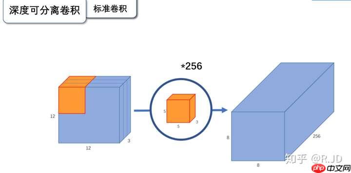
输入一个12×12×3的一个输入特征图,经过5×5×3的卷积核卷积得到一个8×8×1的输出特征图。如果此时我们有256个特征图,我们将会得到一个8×8×256的输出特征图。
以上就是标准卷积做干的活。那深度卷积和逐点卷积呢?

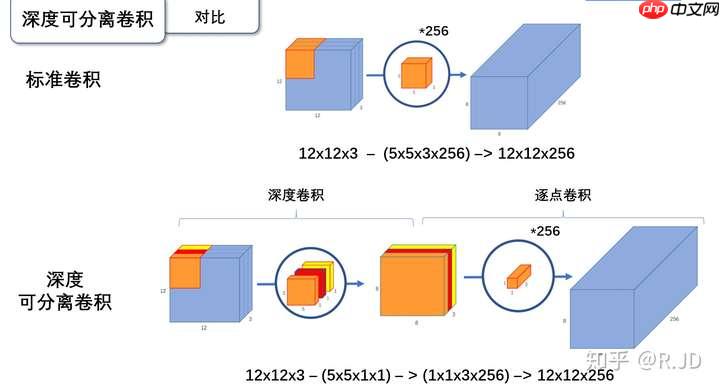
与标准卷积网络不一样的是,我们将卷积核拆分成为但单通道形式,在不改变输入特征图像的深度的情况下,对每一通道进行卷积操作,这样就得到了和输入特征图通道数一致的输出特征图。如上图:输入12×12×3的特征图,经过5×5×1×3的深度卷积之后,得到了8×8×3的输出特征图。输入个输出的维度是不变的3。这样就会有一个问题,通道数太少,特征图的维度太少,能获取到足够的有效信息吗?
逐点卷积就是1×1卷积。主要作用就是对特征图进行升维和降维,如下图:

在深度卷积的过程中,我们得到了8×8×3的输出特征图,我们用256个1×1×3的卷积核对输入特征图进行卷积操作,输出的特征图和标准的卷积操作一样都是8×8×256了。
标准卷积与深度可分离卷积的过程对比如下:
应该为12x13x3---(5x5x1x3)--(1x1x3x256)-->12x12x256。
这个问题很好回答,如果有一个方法能让你用更少的参数,更少的运算,但是能达到差的不是很多的结果,你会使用吗?
深度可分离卷积就是这样的一个方法。
深度可分离卷积的参数量由深度卷积和逐点卷积两部分组成:
这一层,MobileNetV1所采用的深度可分离卷积计算量与标准卷积计算量的比值为:
109985792 /924844032 = 0.1189
与我们所计算的九分之一到八分之一一致。
V1卷积层

上图左边是标准卷积层,右边是V1的卷积层,虚线处是不相同点。V1的卷积层,首先使用3×3的深度卷积提取特征,接着是一个BN层,随后是一个ReLU层,在之后就会逐点卷积,最后就是BN和ReLU了。这也很符合深度可分离卷积,将左边的标准卷积拆分成右边的一个深度卷积和一个逐点卷积。
等等,我们发现有什么东西混了进来???ReLU6是什么?
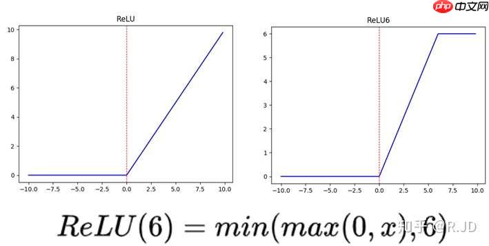
上图左边是普通的ReLU,对于大于0的值不进行处理,右边是ReLU6,当输入的值大于6的时候,返回6,relu6“具有一个边界”。作者认为ReLU6作为非线性激活函数,在低精度计算下具有更强的鲁棒性。(这里所说的“低精度”,我看到有人说不是指的float16,而是指的定点运算(fixed-point arithmetic))
可以看到使用深度可分离卷积与标准卷积,参数和计算量能下降为后者的九分之一到八分之一左右。但是准确率只有下降极小的1%。
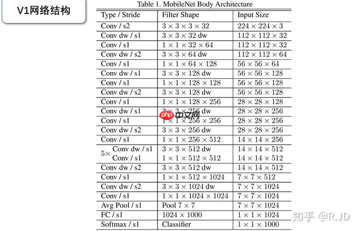
MobileNet的网络结构如上图所示。首先是一个3x3的标准卷积,s2进行下采样。然后就是堆积深度可分离卷积,并且其中的部分深度卷积会利用s2进行下采样。然后采用平均池化层将feature变成1x1,根据预测类别大小加上全连接层,最后是一个softmax层。整个网络有28层,其中深度卷积层有13层。

可以发现,作为轻量级网络的V1在计算量小于GoogleNet,参数量差不多是在一个数量级的基础上,在分类效果上比GoogleNet还要好,这就是要得益于深度可分离卷积了。VGG16的计算量参数量比V1大了30倍,但是结果也仅仅只高了1%不到。
对了,作者还在论文中分析整个了网络的参数和计算量分布,如下图所示。可以看到整个计算量基本集中在1x1卷积上。对于参数也主要集中在1x1卷积,除此之外还有就是全连接层占了一部分参数。

torch.nn.Conv2d:对输入的二维图像进行卷积运算
以2 x 3 x 4 x 5 input为例
此时卷积核shape为 6 x 3 x 3 x 3 [out_channels x in_channels x kernel_size x kernel_size] 此时groups参数为1,表示将in_channels所有通道作为一组,与每一个3x3x3卷积核卷积,一共6个3x3x3卷积核,共输出6个通道特征
先大概总结一下groups参数的含义:假设卷积操作的输入通道数是in_channels,输出通道数是out_channles,分组数是groups,分组卷积就是把原本的整体卷积操作分成groups个小组来分别处理,其中每个分组的输入通道数是in_channles / groups,输出通道数是out_channles / groups,最后将所有分组的输出通道数concat,得到最终的输出通道数out_channles,所以在做分组卷积的时候,in_channels和out_channels需要被groups整除
class MobileNet_v1(nn.Layer):
    def __init__(self):
        super(MobileNet_v1,self).__init__()
        #标准卷积
        def conv_bn(inp,oup,stride):
            return nn.Sequential(                    # stride==1 尺寸不变
                    # stride==2 尺寸减半
                    nn.Conv2D(inp,oup,3,stride,1,bias_attr = False),
                    nn.BatchNorm2D(oup),
                    nn.ReLU())
        #深度卷积
        def conv_dw(inp,oup,stride):
            return nn.Sequential(                    # groups!=1时为深度卷积
                    nn.Conv2D(inp,inp,3,stride,1,groups = inp,bias_attr = False),
                    nn.BatchNorm2D(inp),
                    nn.ReLU(),                    # 1*1卷积
                    nn.Conv2D(inp,oup,1,1,0,bias_attr = False),
                    nn.BatchNorm2D(oup),
                    nn.ReLU())
        #网络模型声明
        self.model = nn.Sequential(            #标准卷积
            conv_bn(3,32,2),            #深度卷积
            conv_dw(32,64,1),
            conv_dw(64,128,2),
            conv_dw(128,128,1),
            conv_dw(128,256,2),
            conv_dw(256,256,1),
            conv_dw(256,512,2),
            conv_dw(512,512,1),
            conv_dw(512,512,1),
            conv_dw(512,512,1),
            conv_dw(512,512,1),
            conv_dw(512,512,1),
            conv_dw(512,1024,2),
            conv_dw(1024,1024,1),
            nn.AvgPool2D(7),
        )        # 全连接层
        self.fc = nn.Linear(1024,10)
    #网络的前向过程
    def forward(self,x):
        x = self.model(x)
        x=paddle.reshape(x,[-1, 1024])
x = self.fc(x) return x在MobileNet v1的网络结构表中能够发现,网络的结构就像VGG一样是个直筒型的,不像ResNet网络有shorcut之类的连接方式。而且有人反映说MobileNet v1网络中的DW卷积很容易训练废掉,效果并没有那么理想。所以我们接着看下MobileNet v2网络。
MobileNet v2网络是由google团队在2018年提出的,相比MobileNet V1网络,准确率更高,模型更小。

刚刚说了MobileNet v1网络中的亮点是DW卷积,那么在MobileNet v2中的亮点就是Inverted residual block(倒残差结构),同时分析了v1的几个缺点并针对性的做了改进
在进行完卷积操作之后往往会接一层激活函数来增加特征的非线性性,一个最常见的激活函数便是ReLU。根据我们在残差网络中介绍的数据处理不等式(DPI),ReLU一定会带来信息损耗,而且这种损耗是没有办法恢复的,ReLU的信息损耗是当通道数非常少的时候更为明显。

在残差结构中是1x1卷积降维->3x3卷积->1x1卷积升维,在倒残差结构中正好相反,是1x1卷积升维->3x3DW卷积->1x1卷积降维。为什么要这样做,原文的解释是高维信息通过ReLU激活函数后丢失的信息更少(注意倒残差结构中基本使用的都是ReLU6激活函数,但是最后一个1x1的卷积层使用的是线性激活函数)。
在使用倒残差结构时需要注意下,并不是所有的倒残差结构都有shortcut连接,只有当stride=1且输入特征矩阵与输出特征矩阵shape相同时才有shortcut连接(只有当shape相同时,两个矩阵才能做加法运算,当stride=1时并不能保证输入特征矩阵的channel与输出特征矩阵的channel相同)。
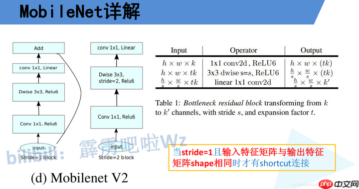
下图是MobileNet v2网络的结构表,其中t代表的是扩展因子(倒残差结构中第一个1x1卷积的扩展因子),c代表输出特征矩阵的channel,n代表倒残差结构重复的次数,s代表步距(注意:这里的步距只是针对重复n次的第一层倒残差结构,后面的都默认为1)。
因为MobileNet 网络结构的核心就是Depth-wise,此卷积方式可以减少计算量和参数量。而为了引入shortcut结构,若参照Resnet中先压缩特征图的方式,将使输入给Depth-wise的特征图大小太小,接下来可提取的特征信息少,所以在MobileNet V2中采用先扩张后压缩的策略。
因为在激活函数之前,已经使用1*1卷积对特征图进行了压缩,而ReLu激活函数对于负的输入值,输出为0,会进一步造成信息的损失,所以使用Linear激活函数。
MobileNet v1最主要的贡献是使用了Depthwise Separable Convolution,它又可以拆分成Depthwise卷积和Pointwise卷积。MobileNet v2主要是将残差网络和Depthwise Separable卷积进行了结合。通过分析单通道的流形特征对残差块进行了改进,包括对中间层的扩展(d)以及bottleneck层的线性激活(c)。Depthwise Separable Convolution的分离式设计直接将模型压缩了8倍左右,但是精度并没有损失非常严重,这一点还是非常震撼的。
Depthwise Separable卷积的设计非常精彩但遗憾的是目前cudnn对其的支持并不好,导致在使用GPU训练网络过程中我们无法从算法中获益,但是使用串行CPU并没有这个问题,这也就给了MobileNet很大的市场空间,尤其是在嵌入式平台。
# 带倒残差的深度可分离卷积class Bottleneck(nn.Layer):
    def __init__(self, in_channels, out_channels, multiple, stride):
        super(Bottleneck, self).__init__()
        self.stride = stride        # 1*1卷积升维
        self.conv1 = nn.Conv2D(
            in_channels=in_channels,
            out_channels=in_channels*multiple,
            kernel_size=1,
            stride=1,
            padding=0
        )
        self.bn1 = nn.BatchNorm2D(in_channels*multiple)        # 深度卷积
        self.conv2 = nn.Conv2D(
            in_channels=in_channels*multiple,
            out_channels=in_channels*multiple,
            kernel_size=3,
            stride=stride,
            padding=1,
            groups=in_channels*multiple,
        )
        self.bn2 = nn.BatchNorm2D(in_channels*multiple)        # 1*1卷积降维度
        self.conv3 = nn.Conv2D(
            in_channels=in_channels*multiple,
            out_channels=out_channels,
            kernel_size=1,
            stride=1,
            padding=0
        )
        self.bn3 = nn.BatchNorm2D(out_channels)
        self.shortcut = nn.Sequential()        if  in_channels!=out_channels and stride==1:            # 由于stride==1,shape一致,可以做残差连接 即总体上为倒残差结构
            self.shortcut = nn.Sequential(                # 1*1调整shortcut部分通道数
                nn.Conv2D(
                    in_channels=in_channels,
                    out_channels=out_channels,
                    kernel_size=1,
                    stride=1,
                    padding=0
                ),
                nn.BatchNorm2D(out_channels),
            )    def forward(self, x):
        out = F.relu6(self.bn1(self.conv1(x)))
        out = F.relu6(self.bn2(self.conv2(out)))        # 最后一层采用线性激活函数
        out = self.bn3(self.conv3(out))        # 如果stride==1,故shape一致,可以做残差连接 即总体上为倒残差结构
        if self.stride==1:
            out = out + self.shortcut(x)        return outclass MobileNet_v2(nn.Layer):
    parameters = [
        (1,16,1,1),
        (6,24,2,2),
        (6,32,3,2),
        (6,64,4,2),
        (6,96,3,1),
        (6,160,3,2),
        (6,320,1,1)]    def __init__(self,num_classes=10):
        super(MobileNet_v2,self).__init__()
        self.conv1 = nn.Conv2D(
            in_channels=3,
            out_channels=32,
            kernel_size=3,
            stride=1,
            padding=1
        )
        self.bn1 = nn.BatchNorm2D(32)
        self.bottleneck = self.Make_Bottleneck()
        self.conv2 = nn.Conv2D(
            in_channels=320,
            out_channels=1280,
            kernel_size=1,
            stride=1,
            padding=0
        )
        self.bn2 = nn.BatchNorm2D(1280)
        self.linear = nn.Linear(1280,num_classes)    def Make_Bottleneck(self):
        layers = []
        in_channels = 32
        for parameter in self.parameters:
            strides = [parameter[3]] + [1]*(parameter[2]-1)            for stride in strides:
                layer = Bottleneck(in_channels, parameter[1], parameter[0], stride)
                layers.append(layer)
                in_channels = parameter[1]        return nn.Sequential(*layers)    def forward(self, x):
        out = F.relu6(self.bn1(self.conv1(x)))
        out = self.bottleneck(out)
        out = F.relu6(self.bn2(self.conv2(out)))
        out = F.avg_pool2d(out, 4)
        out = F.avg_pool2d(out, 3)
        out=paddle.reshape(out,[out.shape[0], -1])
out = self.linear(out) return out#速度评估def speed(model,name):
t0 = time.time() input = paddle.rand([1,3,224,224])
t1 = time.time()
model(input)
t2 = time.time()
model(input)
t3 = time.time()
print('%10s : %fs'%(name,t3 - t2))resnet50
resnet152
vgg16
vgg19
mobilenet_v1
mobilenet_v2
resnet50 = models.resnet50()
resnet152 = models.resnet152()
vgg16 = models.vgg16()
vgg19 = models.vgg19()
mobilenet_v1 = MobileNet_v1()
mobilenet_v2 = MobileNet_v2()

speed(resnet50,'resnet50')
speed(resnet152,'resnet152')
speed(vgg16,'vgg16')
speed(vgg19,'vgg19')
speed(mobilenet_v1,'mobilenet_v1')
speed(mobilenet_v2,'mobilenet_v2')
resnet50 : 0.019720s
resnet152 : 0.058257s
vgg16 : 0.004025s
vgg19 : 0.004707s
mobilenet_v1 : 0.008120s
mobilenet_v2 : 0.020288s
可能是因为参数量的不同,导致速度有些差异,也与硬件环境有关,在本地运行时,无论是mobilenet_v1,还是mobilenet_v2,均要比vgg网络快
使用Cifar10数据集测试MobileNet_v1,MobileNet_v2的精度
transform_train = Compose([
    transforms.Resize([224, 224]),
    transforms.ToTensor(),
    transforms.Normalize([0.485, 0.456, 0.406], [0.229, 0.224, 0.225]),
])

transform_test = Compose([
    transforms.Resize([224, 224]),
    transforms.ToTensor(),
    transforms.Normalize([0.485, 0.456, 0.406], [0.229, 0.224, 0.225]),
])

LR = 0.001EPOCHES = 3BATCHSIZE = 100trainset=Cifar10(data_file=None, mode='train', transform=transform_train, download=True)
testset=Cifar10(data_file=None, mode='test', transform=transform_test, download=True)

trainloader = paddle.io.DataLoader(trainset, batch_size=BATCHSIZE, shuffle=True, num_workers=2)
testloader = paddle.io.DataLoader(testset, batch_size=BATCHSIZE, shuffle=False, num_workers=2)mobilenet_v1 = MobileNet_v1()
optimizer = paddle.optimizer.Adam(learning_rate=LR,parameters=mobilenet_v1.parameters())
loss_function = nn.CrossEntropyLoss()for ep in range(EPOCHES):
train_correct = 0
train_sum=0
epoch_used_time=0
epoch_ave_time=0
time_start=time.time() for i,(img, label) in enumerate(trainloader):
optimizer.clear_grad()
mobilenet_v1.train()
out = mobilenet_v1(img)
prediction = paddle.argmax(out, 1)
pre_num = prediction.cpu().numpy()
train_correct += (pre_num == label.cpu().numpy()).sum()
train_sum+=BATCHSIZE
loss = loss_function(out, label)
loss.backward()
optimizer.step()
epoch_used_time+=(time.time()-time_start)
time_start=time.time()
used_t=strftime("%H:%M:%S", gmtime(epoch_used_time))
total_t=strftime("%H:%M:%S", gmtime((epoch_used_time/(i+1))*len(trainloader))) print(f"\rEpoch:{str(ep)} Iter {train_sum}/{len(trainloader)*BATCHSIZE} Train ACC: {(train_correct/train_sum):.5}\
Used_Time:{used_t} / Total_Time:{total_t}",end="")
print('')
vote_correct = 0
test_sum=0
for img, label in testloader:
mobilenet_v1.eval()
out = mobilenet_v1(img)
prediction = paddle.argmax(out, 1)
pre_num = prediction.cpu().numpy()
vote_correct += (pre_num == label.cpu().numpy()).sum()
test_sum+=BATCHSIZE
print(f"\rEpoch:{str(ep)} Iter {test_sum}/{len(testloader)*BATCHSIZE} Test ACC: {(vote_correct/test_sum):.5}",end="") print('')mobilenet_v1 3 Epoch 效果
Epoch:0 Iter 50000/50000 Train ACC: 0.47304 Used_Time:00:01:37 / Total_Time:00:01:37
Epoch:0 Iter 10000/10000 Test ACC: 0.5915
Epoch:1 Iter 50000/50000 Train ACC: 0.65172 Used_Time:00:01:39 / Total_Time:00:01:39
Epoch:1 Iter 10000/10000 Test ACC: 0.6733
Epoch:2 Iter 50000/50000 Train ACC: 0.73912 Used_Time:00:01:40 / Total_Time:00:01:40
Epoch:2 Iter 10000/10000 Test ACC: 0.7497
from paddle.vision.models import mobilenet_v2

mobilenet_v2 = mobilenet_v2(pretrained=False)
optimizer_v2 = paddle.optimizer.Adam(learning_rate=LR,parameters=mobilenet_v2.parameters())
loss_function = nn.CrossEntropyLoss()for ep in range(EPOCHES):
    train_correct = 0
    train_sum=0
    epoch_used_time=0
    epoch_ave_time=0
    time_start=time.time()    for i,(img, label) in enumerate(trainloader):

        optimizer_v2.clear_grad()
        mobilenet_v2.train()
        out = mobilenet_v2(img)

        prediction = paddle.argmax(out, 1)
        pre_num = prediction.cpu().numpy()
        train_correct += (pre_num == label.cpu().numpy()).sum()
        train_sum+=BATCHSIZE

        loss = loss_function(out, label)
        loss.backward()
        optimizer_v2.step()

        epoch_used_time+=(time.time()-time_start)
        time_start=time.time()

        used_t=strftime("%H:%M:%S", gmtime(epoch_used_time))
        total_t=strftime("%H:%M:%S", gmtime((epoch_used_time/(i+1))*len(trainloader)))        print(f"\rEpoch:{str(ep)} Iter {train_sum}/{len(trainloader)*BATCHSIZE} Train ACC: {(train_correct/train_sum):.5}\
    Used_Time:{used_t} / Total_Time:{total_t}",end="")
    print('')

    vote_correct = 0
    test_sum=0
    for img, label in testloader:
        mobilenet_v2.eval()
        out = mobilenet_v2(img)
        prediction = paddle.argmax(out, 1)
        pre_num = prediction.cpu().numpy()
        vote_correct += (pre_num == label.cpu().numpy()).sum()
        test_sum+=BATCHSIZE
print(f"\rEpoch:{str(ep)} Iter {test_sum}/{len(testloader)*BATCHSIZE} Test ACC: {(vote_correct/test_sum):.5}",end="") print('')mobilenet_v2 3 Epoch 效果
Epoch:0 Iter 50000/50000 Train ACC: 0.50066 Used_Time:00:01:43 / Total_Time:00:01:43
Epoch:0 Iter 10000/10000 Test ACC: 0.5784
Epoch:1 Iter 50000/50000 Train ACC: 0.6868 Used_Time:00:01:43 / Total_Time:00:01:433
Epoch:1 Iter 10000/10000 Test ACC: 0.7133
Epoch:2 Iter 50000/50000 Train ACC: 0.76648 Used_Time:00:01:43 / Total_Time:00:01:43
Epoch:2 Iter 10000/10000 Test ACC: 0.7486
net = models.resnet50(pretrained=False)
optimizer = paddle.optimizer.Adam(learning_rate=LR,parameters=net.parameters())
loss_function = nn.CrossEntropyLoss()for ep in range(EPOCHES):
    train_correct = 0
    train_sum=0
    epoch_used_time=0
    epoch_ave_time=0
    time_start=time.time()    for i,(img, label) in enumerate(trainloader):

        optimizer.clear_grad()
        net.train()
        out = net(img)

        prediction = paddle.argmax(out, 1)
        pre_num = prediction.cpu().numpy()
        train_correct += (pre_num == label.cpu().numpy()).sum()
        train_sum+=BATCHSIZE

        loss = loss_function(out, label)
        loss.backward()
        optimizer.step()

        epoch_used_time+=(time.time()-time_start)
        time_start=time.time()

        used_t=strftime("%H:%M:%S", gmtime(epoch_used_time))
        total_t=strftime("%H:%M:%S", gmtime((epoch_used_time/(i+1))*len(trainloader)))        print(f"\rEpoch:{str(ep)} Iter {train_sum}/{len(trainloader)*BATCHSIZE} Train ACC: {(train_correct/train_sum):.5}\
    Used_Time:{used_t} / Total_Time:{total_t}",end="")
    print(' ')    print(' ')

    vote_correct = 0
    test_sum=0
    for img, label in testloader:
        net.eval()
        out = net(img)
        prediction = paddle.argmax(out, 1)
        pre_num = prediction.cpu().numpy()
        vote_correct += (pre_num == label.cpu().numpy()).sum()
        test_sum+=BATCHSIZE
print(f"\rEpoch:{str(ep)} Iter {test_sum}/{len(testloader)*BATCHSIZE} Test ACC: {(vote_correct/test_sum):.5}",end="") print(' ') print(' ')| mobilenet_v1 | mobilenet_v2 | vgg16 | vgg19 | resnet50 | resnet152 | |
|---|---|---|---|---|---|---|
| 训练集精度 | 0.73912 | 0.76648 | 0.67516 | 0.69153 | 0.74648 | 0.68296 |
| 测试集精度 | 0.7497 | 0.7486 | 0.7027 | 0.71897 | 0.72132 | 0.67154 |
| 1个epoch训练时间 | 1:40min | 1:43min | 5:10min | 6:30min | 2.13min | 5.47min |
可见mobilenet_v2与mobilenet_v1训练所用时间差不多,但是mobilenet_v2的拟合能力更强,且最终的泛化表现也较好
<br/>
以上就是MobileNet_v1_v2论文复现,附带与ResNet,VGG网络对比的详细内容,更多请关注php中文网其它相关文章!

每个人都需要一台速度更快、更稳定的 PC。随着时间的推移,垃圾文件、旧注册表数据和不必要的后台进程会占用资源并降低性能。幸运的是,许多工具可以让 Windows 保持平稳运行。

Copyright 2014-2025 https://www.php.cn/ All Rights Reserved | php.cn | 湘ICP备2023035733号


 806
806