本教程将带领大家从0开始,学习如何使用深度学习模型进行时序预测,以股票价格预测为实战案例。通过本教程,希望您将掌握从数据收集、模型构建到预测分析的完整流程。
☞☞☞AI 智能聊天, 问答助手, AI 智能搜索, 免费无限量使用 DeepSeek R1 模型☜☜☜

本教程将系统全面地讲解如何运用深度学习技术搭建股票预测系统,带领学习者从零基础逐步掌握完整的实现流程。课程内容覆盖数据获取、特征工程、模型构建、预测分析四大核心环节,每个环节都将进行细致的技术实现讲解,确保学习者能够理解并掌握每个步骤的原理和操作方法。项目基于PaddlePaddle深度学习框架,实现了融合注意力机制、残差连接和集成学习的先进预测模型,帮助学习者在实战中提升AI模型构建和应用能力。
aistudio/
├── data_collector.py    # 负责数据采集与预处理,包含多市场数据获取、智能重试机制和特征工程等功能  ├── stock_predictor.py   # 实现预测模型,包括注意力机制、增强型LSTM模型和集成学习等关键技术  ├── visualization.py     # 用于可视化分析,生成交互式图表展示预测结果和市场数据  └── requirements.txt     # 记录项目所需的依赖库,方便环境配置
def get_stock_data(self, ticker, start_date, end_date, market='US', max_retries=3):
    """支持多市场数据获取,包含重试机制"""
    for attempt in range(max_retries):
        try:
            if market == 'US':
                data = self._get_us_stock_data(ticker, start_date, end_date)
            elif market == 'CN':
                data = self._get_cn_stock_data(ticker, start_date, end_date)

            if data is not None and not data.empty:
                return data

            # 智能重试机制
            if attempt < max_retries - 1:
                wait_time = (attempt + 1) * 2 + random.uniform(0, 1)
                time.sleep(wait_time)
技术要点:
def preprocess_data(self, data, seq_length=30, features=None):
    """高级特征预处理"""
    if features is None:
        # 基础特征处理
        close_prices = data['Close'].values.reshape(-1, 1)
        scaled_data = self.scaler.fit_transform(close_prices)
    else:
        # 多维度特征处理
        scaled_data = self.scaler.fit_transform(features)

    # 序列化处理
    x, y = [], []
    for i in range(len(scaled_data) - seq_length):
        x.append(scaled_data[i:i+seq_length])
        y.append(scaled_data[i+seq_length, 0])
技术要点:
class AttentionLayer(nn.Layer):
    """注意力层实现"""
    def __init__(self, hidden_size: int):
        super(AttentionLayer, self).__init__()
        self.attention = nn.Sequential(
            nn.Linear(hidden_size, hidden_size),
            nn.Tanh(),
            nn.Linear(hidden_size, 1)
        )

    def forward(self, lstm_output):
        # 计算注意力权重
        attention_weights = self.attention(lstm_output)
        attention_weights = paddle.nn.functional.softmax(attention_weights, axis=0)
        # 加权求和
        context = paddle.sum(attention_weights * lstm_output, axis=0)
        return context, attention_weights
技术要点:
class EnhancedLSTMModel(nn.Layer):
    """增强版LSTM模型"""
    def __init__(self, input_size=35, hidden_size=64,
                 num_layers=2, output_size=1, dropout=0.2):
        super(EnhancedLSTMModel, self).__init__()

        # 多层LSTM
        self.lstm_layers = nn.LayerList([
            nn.LSTM(
                input_size if i == 0 else hidden_size,
                hidden_size,
                time_major=True
            ) for i in range(num_layers)
        ])

        # 注意力层
        self.attention = AttentionLayer(hidden_size)

        # 残差连接
        self.residual = nn.Linear(input_size, hidden_size)

        # Dropout层
        self.dropout = nn.Dropout(dropout)
技术要点:
class EnsemblePredictor:
    """集成预测器"""
    def __init__(self, models: List[nn.Layer], weights: Optional[List[float]] = None):
        self.models = models
        self.weights = weights if weights is not None else [1.0/len(models)] * len(models)

    def predict(self, x: paddle.Tensor) -> paddle.Tensor:
        """集成预测"""
        predictions = []
        for model, weight in zip(self.models, self.weights):
            with paddle.no_grad():
                pred = model(x)
                predictions.append(pred * weight)
        return paddle.sum(paddle.stack(predictions), axis=0)
技术要点:
class TechnicalIndicators:
    """技术指标计算"""      @staticmethod
    def calculate_macd(prices: np.ndarray, fast_period=12,
                      slow_period=26, signal_period=9):
        """MACD指标计算"""
        prices_series = pd.Series(prices)
        exp1 = prices_series.ewm(span=fast_period, adjust=False).mean()
        exp2 = prices_series.ewm(span=slow_period, adjust=False).mean()
        macd = exp1 - exp2
        signal = macd.ewm(span=signal_period, adjust=False).mean()
        hist = macd - signal
        return macd.values, signal.values, hist.values
技术要点:
class MarketSentimentAnalyzer:
    """市场情绪分析"""
    def calculate_money_flow_index(self, high, low, close, volume, period=14):
        """资金流量指标计算"""
        typical_price = (high + low + close) / 3
        money_flow = typical_price * volume

        positive_flow = np.zeros_like(money_flow)
        negative_flow = np.zeros_like(money_flow)

        for i in range(1, len(money_flow)):
            if typical_price[i] > typical_price[i-1]:
                positive_flow[i] = money_flow[i]
            else:
                negative_flow[i] = money_flow[i]
技术要点:
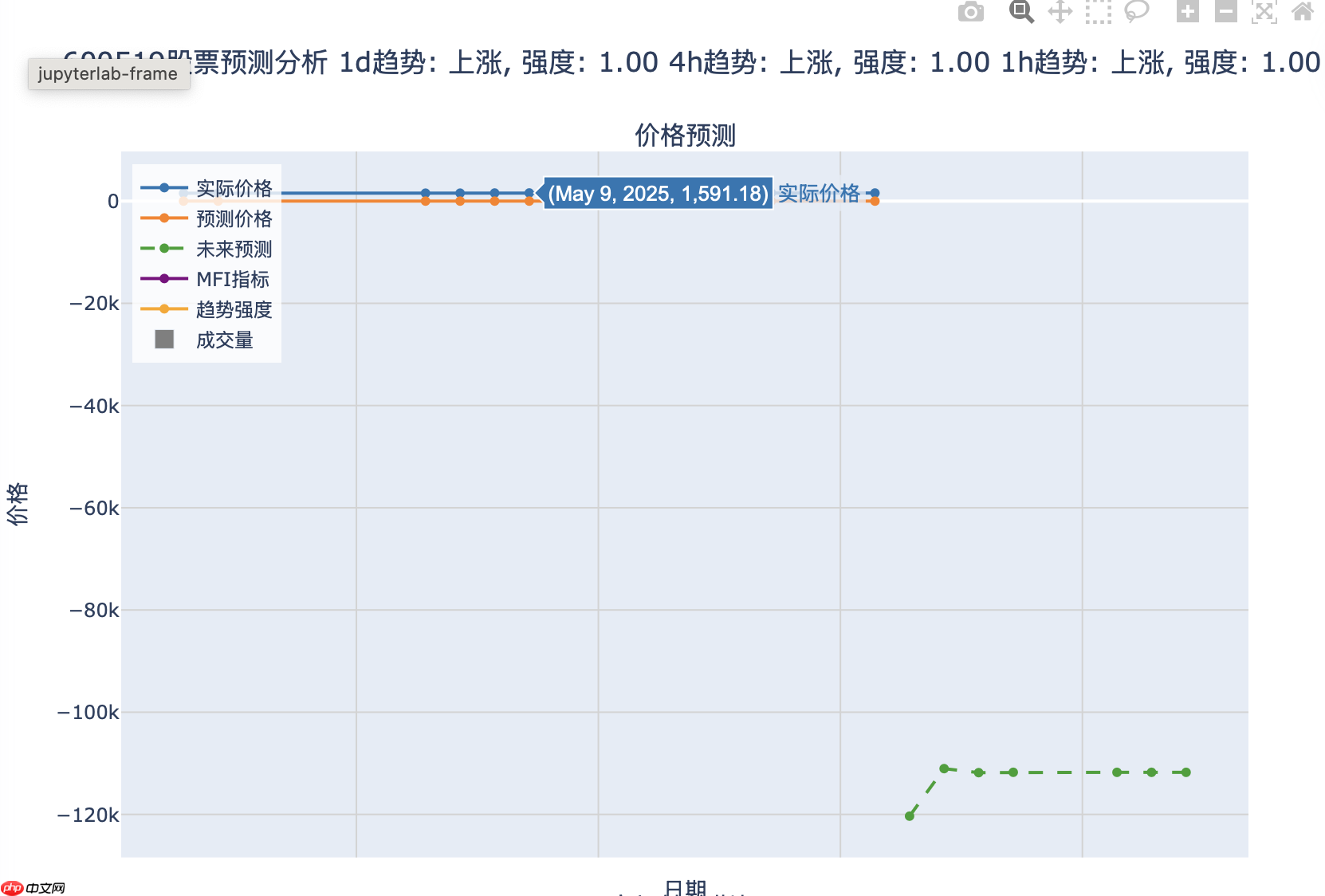
def plot_stock_prediction(self, data, predictions, future_predictions,
market_conditions, title="股票预测分析"):
"""交互式预测分析图表"""
fig = make_subplots(
rows=3, cols=1,
shared_xaxes=True,
vertical_spacing=0.05,
row_heights=[0.6, 0.2, 0.2],
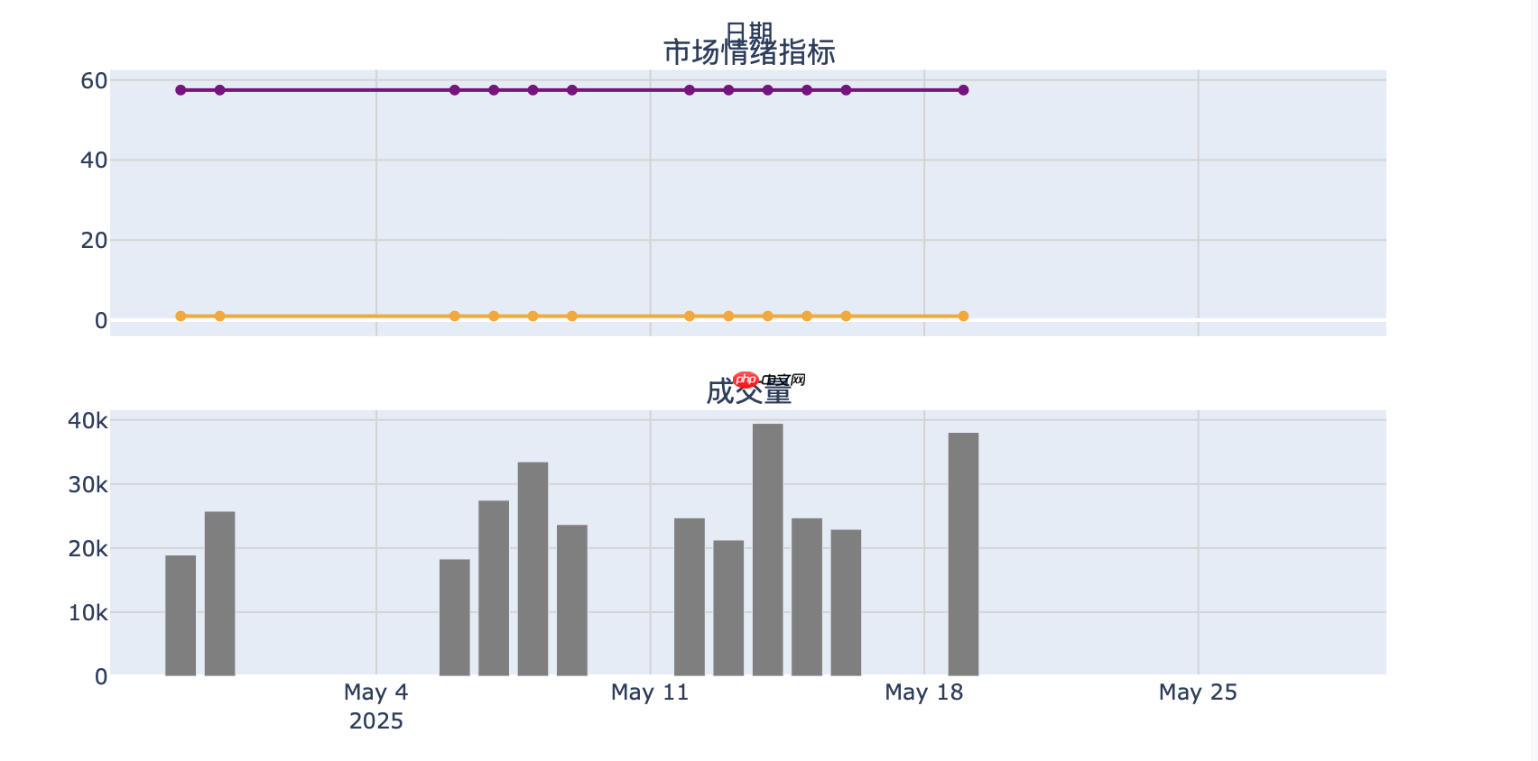
subplot_titles=("价格预测", "市场情绪指标", "成交量")
)
# 添加价格预测
fig.add_trace(
go.Scatter(
x=data.index[-len(predictions):],
y=predictions,
name='预测价格',
line=dict(color=self.colors['predicted'])
),
row=1, col=1
)
技术要点:
# 安装依赖 pip install -r requirements.txt # 根据requirements.txt文件安装项目所需的依赖库
python stock_predictor.py
#示例开始批量分析股票...

开始批量分析 20 只股票...

分析 贵州茅台(600519)...
正在获取 600519 的A股数据...
成功获取 600519 的数据,共 88 个交易日

市场状况分析:
趋势强度: 1.00
MFI指标: 57.48
特征维度检查:
technical_features shape: (88, 15)
sentiment_features shape: (88, 11)
timeframe_features shape: (88, 9)

开始训练模型...
开始训练,数据集大小: 46
输入特征维度: 35
W0519 19:16:50.071368 263776 gpu_resources.cc:306] WARNING: device: 0. The installed Paddle is compiled with CUDNN 8.9, but CUDNN version in your machine is 8.9, which may cause serious incompatible bug. Please recompile or reinstall Paddle with compatible CUDNN version.
Epoch [10/100], Average Loss: 0.177549
Epoch [20/100], Average Loss: 0.068324
Epoch [30/100], Average Loss: 0.042560
Epoch [40/100], Average Loss: 0.031994
Epoch [50/100], Average Loss: 0.030030
Epoch [60/100], Average Loss: 0.034403
Epoch [70/100], Average Loss: 0.025163
Epoch [80/100], Average Loss: 0.023011
Epoch [90/100], Average Loss: 0.026051
Epoch [100/100], Average Loss: 0.021419

评估模型性能...
开始评估,测试集大小: 12

预测未来价格...
特征维度检查:
technical_features shape: (88, 15)
sentiment_features shape: (88, 11)
timeframe_features shape: (88, 9)

生成可视化结果...
通过本教程的学习,希望您将掌握构建股票预测系统的完整技能,并能够将这些技术应用到实际的量化交易场景中。让我们开始这个深度学习之旅,探索AI在股票预测领域的无限可能!
%%capture
!pip install yfinance akshare plotly textblob optuna
!python stock_predictor.py
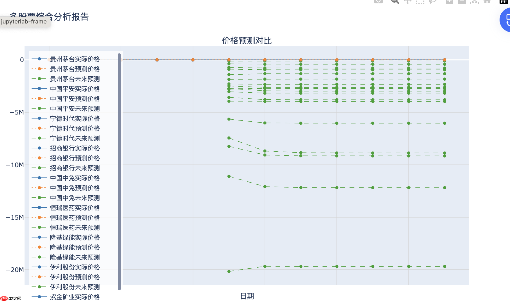
/opt/conda/envs/python35-paddle120-env/lib/python3.10/site-packages/paddle/utils/cpp_extension/extension_utils.py:711: UserWarning: No ccache found. Please be aware that recompiling all source files may be required. You can download and install ccache from: https://github.com/ccache/ccache/blob/master/doc/INSTALL.md
  warnings.warn(warning_message)
W0519 19:16:37.067554 263776 gpu_resources.cc:119] Please NOTE: device: 0, GPU Compute Capability: 7.0, Driver API Version: 12.0, Runtime API Version: 11.8
W0519 19:16:37.068797 263776 gpu_resources.cc:164] device: 0, cuDNN Version: 8.9.
开始批量分析股票...

开始批量分析 20 只股票...

分析 贵州茅台(600519)...
正在获取 600519 的A股数据...
成功获取 600519 的数据,共 88 个交易日

市场状况分析:
趋势强度: 1.00
MFI指标: 57.48
特征维度检查:
technical_features shape: (88, 15)
sentiment_features shape: (88, 11)
timeframe_features shape: (88, 9)

开始训练模型...
开始训练,数据集大小: 46
输入特征维度: 35
W0519 19:16:50.071368 263776 gpu_resources.cc:306] WARNING: device: 0. The installed Paddle is compiled with CUDNN 8.9, but CUDNN version in your machine is 8.9, which may cause serious incompatible bug. Please recompile or reinstall Paddle with compatible CUDNN version.
Epoch [10/100], Average Loss: 0.177549
Epoch [20/100], Average Loss: 0.068324
Epoch [30/100], Average Loss: 0.042560
Epoch [40/100], Average Loss: 0.031994
Epoch [50/100], Average Loss: 0.030030
Epoch [60/100], Average Loss: 0.034403
Epoch [70/100], Average Loss: 0.025163
Epoch [80/100], Average Loss: 0.023011
Epoch [90/100], Average Loss: 0.026051
Epoch [100/100], Average Loss: 0.021419

评估模型性能...
开始评估,测试集大小: 12

预测未来价格...
特征维度检查:
technical_features shape: (88, 15)
sentiment_features shape: (88, 11)
timeframe_features shape: (88, 9)

生成可视化结果...

分析 中国平安(601318)...
正在获取 601318 的A股数据...
成功获取 601318 的数据,共 88 个交易日

市场状况分析:
趋势强度: 1.06
MFI指标: 71.84
特征维度检查:
technical_features shape: (88, 15)
sentiment_features shape: (88, 11)
timeframe_features shape: (88, 9)

开始训练模型...
开始训练,数据集大小: 46
输入特征维度: 35
Epoch [10/100], Average Loss: 0.025576
Epoch [20/100], Average Loss: 0.026208
Epoch [30/100], Average Loss: 0.016376
Epoch [40/100], Average Loss: 0.020805
Epoch [50/100], Average Loss: 0.022497
Epoch [60/100], Average Loss: 0.018886
Epoch [70/100], Average Loss: 0.019082
Epoch [80/100], Average Loss: 0.013531
Epoch [90/100], Average Loss: 0.012390
Epoch [100/100], Average Loss: 0.025220

评估模型性能...
开始评估,测试集大小: 12

预测未来价格...
特征维度检查:
technical_features shape: (88, 15)
sentiment_features shape: (88, 11)
timeframe_features shape: (88, 9)

生成可视化结果...

分析 宁德时代(300750)...
正在获取 300750 的A股数据...
成功获取 300750 的数据,共 88 个交易日

市场状况分析:
趋势强度: 1.11
MFI指标: 66.60
特征维度检查:
technical_features shape: (88, 15)
sentiment_features shape: (88, 11)
timeframe_features shape: (88, 9)

开始训练模型...
开始训练,数据集大小: 46
输入特征维度: 35
Epoch [10/100], Average Loss: 0.032299
Epoch [20/100], Average Loss: 0.020735
Epoch [30/100], Average Loss: 0.019277
Epoch [40/100], Average Loss: 0.021626
Epoch [50/100], Average Loss: 0.012644
Epoch [60/100], Average Loss: 0.017141
Epoch [70/100], Average Loss: 0.016274
Epoch [80/100], Average Loss: 0.014255
Epoch [90/100], Average Loss: 0.012987
Epoch [100/100], Average Loss: 0.014642

评估模型性能...
开始评估,测试集大小: 12

预测未来价格...
特征维度检查:
technical_features shape: (88, 15)
sentiment_features shape: (88, 11)
timeframe_features shape: (88, 9)

生成可视化结果...

分析 招商银行(600036)...
正在获取 600036 的A股数据...
成功获取 600036 的数据,共 88 个交易日

市场状况分析:
趋势强度: 1.07
MFI指标: 71.03
特征维度检查:
technical_features shape: (88, 15)
sentiment_features shape: (88, 11)
timeframe_features shape: (88, 9)

开始训练模型...
开始训练,数据集大小: 46
输入特征维度: 35
Epoch [10/100], Average Loss: 0.016462
Epoch [20/100], Average Loss: 0.014358
Epoch [30/100], Average Loss: 0.015646
Epoch [40/100], Average Loss: 0.013511
Epoch [50/100], Average Loss: 0.015170
Epoch [60/100], Average Loss: 0.016921
Epoch [70/100], Average Loss: 0.010113
Epoch [80/100], Average Loss: 0.011124
Epoch [90/100], Average Loss: 0.011751
Epoch [100/100], Average Loss: 0.011730

评估模型性能...
开始评估,测试集大小: 12

预测未来价格...
特征维度检查:
technical_features shape: (88, 15)
sentiment_features shape: (88, 11)
timeframe_features shape: (88, 9)

生成可视化结果...

分析 中国中免(601888)...
正在获取 601888 的A股数据...
成功获取 601888 的数据,共 88 个交易日

市场状况分析:
趋势强度: 0.91
MFI指标: 57.02
特征维度检查:
technical_features shape: (88, 15)
sentiment_features shape: (88, 11)
timeframe_features shape: (88, 9)

开始训练模型...
开始训练,数据集大小: 46
输入特征维度: 35
Epoch [10/100], Average Loss: 0.022442
Epoch [20/100], Average Loss: 0.016663
Epoch [30/100], Average Loss: 0.015412
Epoch [40/100], Average Loss: 0.010937
Epoch [50/100], Average Loss: 0.010318
Epoch [60/100], Average Loss: 0.011960
Epoch [70/100], Average Loss: 0.013766
Epoch [80/100], Average Loss: 0.007836
Epoch [90/100], Average Loss: 0.013162
Epoch [100/100], Average Loss: 0.007295

评估模型性能...
开始评估,测试集大小: 12

预测未来价格...
特征维度检查:
technical_features shape: (88, 15)
sentiment_features shape: (88, 11)
timeframe_features shape: (88, 9)

生成可视化结果...

分析 恒瑞医药(600276)...
正在获取 600276 的A股数据...
成功获取 600276 的数据,共 88 个交易日

市场状况分析:
趋势强度: 0.99
MFI指标: 64.45
特征维度检查:
technical_features shape: (88, 15)
sentiment_features shape: (88, 11)
timeframe_features shape: (88, 9)

开始训练模型...
开始训练,数据集大小: 46
输入特征维度: 35
Epoch [10/100], Average Loss: 0.012634
Epoch [20/100], Average Loss: 0.010266
Epoch [30/100], Average Loss: 0.010295
Epoch [40/100], Average Loss: 0.010261
Epoch [50/100], Average Loss: 0.012651
Epoch [60/100], Average Loss: 0.010695
Epoch [70/100], Average Loss: 0.007714
Epoch [80/100], Average Loss: 0.007552
Epoch [90/100], Average Loss: 0.009198
Epoch [100/100], Average Loss: 0.007885

评估模型性能...
开始评估,测试集大小: 12

预测未来价格...
特征维度检查:
technical_features shape: (88, 15)
sentiment_features shape: (88, 11)
timeframe_features shape: (88, 9)

生成可视化结果...

分析 隆基绿能(601012)...
正在获取 601012 的A股数据...
成功获取 601012 的数据,共 88 个交易日

市场状况分析:
趋势强度: 1.08
MFI指标: 55.84
特征维度检查:
technical_features shape: (88, 15)
sentiment_features shape: (88, 11)
timeframe_features shape: (88, 9)

开始训练模型...
开始训练,数据集大小: 46
输入特征维度: 35
Epoch [10/100], Average Loss: 0.040587
Epoch [20/100], Average Loss: 0.021273
Epoch [30/100], Average Loss: 0.022029
Epoch [40/100], Average Loss: 0.017769
Epoch [50/100], Average Loss: 0.016087
Epoch [60/100], Average Loss: 0.015628
Epoch [70/100], Average Loss: 0.012289
Epoch [80/100], Average Loss: 0.018931
Epoch [90/100], Average Loss: 0.013700
Epoch [100/100], Average Loss: 0.018887

评估模型性能...
开始评估,测试集大小: 12

预测未来价格...
特征维度检查:
technical_features shape: (88, 15)
sentiment_features shape: (88, 11)
timeframe_features shape: (88, 9)

生成可视化结果...

分析 伊利股份(600887)...
正在获取 600887 的A股数据...
成功获取 600887 的数据,共 88 个交易日

市场状况分析:
趋势强度: 0.95
MFI指标: 64.69
特征维度检查:
technical_features shape: (88, 15)
sentiment_features shape: (88, 11)
timeframe_features shape: (88, 9)

开始训练模型...
开始训练,数据集大小: 46
输入特征维度: 35
Epoch [10/100], Average Loss: 0.030780
Epoch [20/100], Average Loss: 0.028689
Epoch [30/100], Average Loss: 0.012141
Epoch [40/100], Average Loss: 0.012537
Epoch [50/100], Average Loss: 0.013843
Epoch [60/100], Average Loss: 0.012547
Epoch [70/100], Average Loss: 0.023255
Epoch [80/100], Average Loss: 0.009912
Epoch [90/100], Average Loss: 0.025595
Epoch [100/100], Average Loss: 0.016800

评估模型性能...
开始评估,测试集大小: 12

预测未来价格...
特征维度检查:
technical_features shape: (88, 15)
sentiment_features shape: (88, 11)
timeframe_features shape: (88, 9)

生成可视化结果...

分析 紫金矿业(601899)...
正在获取 601899 的A股数据...
成功获取 601899 的数据,共 88 个交易日

市场状况分析:
趋势强度: 1.02
MFI指标: 39.17
特征维度检查:
technical_features shape: (88, 15)
sentiment_features shape: (88, 11)
timeframe_features shape: (88, 9)

开始训练模型...
开始训练,数据集大小: 46
输入特征维度: 35
Epoch [10/100], Average Loss: 0.019811
Epoch [20/100], Average Loss: 0.019415
Epoch [30/100], Average Loss: 0.013704
Epoch [40/100], Average Loss: 0.017832
Epoch [50/100], Average Loss: 0.014497
Epoch [60/100], Average Loss: 0.016476
Epoch [70/100], Average Loss: 0.018871
Epoch [80/100], Average Loss: 0.011805
Epoch [90/100], Average Loss: 0.013423
Epoch [100/100], Average Loss: 0.016418

评估模型性能...
开始评估,测试集大小: 12

预测未来价格...
特征维度检查:
technical_features shape: (88, 15)
sentiment_features shape: (88, 11)
timeframe_features shape: (88, 9)

生成可视化结果...

分析 万华化学(600309)...
正在获取 600309 的A股数据...
成功获取 600309 的数据,共 88 个交易日

市场状况分析:
趋势强度: 1.03
MFI指标: 60.32
特征维度检查:
technical_features shape: (88, 15)
sentiment_features shape: (88, 11)
timeframe_features shape: (88, 9)

开始训练模型...
开始训练,数据集大小: 46
输入特征维度: 35
Epoch [10/100], Average Loss: 0.013427
Epoch [20/100], Average Loss: 0.014308
Epoch [30/100], Average Loss: 0.011574
Epoch [40/100], Average Loss: 0.010305
Epoch [50/100], Average Loss: 0.012286
Epoch [60/100], Average Loss: 0.012135
Epoch [70/100], Average Loss: 0.007812
Epoch [80/100], Average Loss: 0.010709
Epoch [90/100], Average Loss: 0.010771
Epoch [100/100], Average Loss: 0.010703

评估模型性能...
开始评估,测试集大小: 12

预测未来价格...
特征维度检查:
technical_features shape: (88, 15)
sentiment_features shape: (88, 11)
timeframe_features shape: (88, 9)

生成可视化结果...

分析 比亚迪(002594)...
正在获取 002594 的A股数据...
成功获取 002594 的数据,共 88 个交易日

市场状况分析:
趋势强度: 1.04
MFI指标: 67.95
特征维度检查:
technical_features shape: (88, 15)
sentiment_features shape: (88, 11)
timeframe_features shape: (88, 9)

开始训练模型...
开始训练,数据集大小: 46
输入特征维度: 35
Epoch [10/100], Average Loss: 0.014990
Epoch [20/100], Average Loss: 0.009275
Epoch [30/100], Average Loss: 0.012158
Epoch [40/100], Average Loss: 0.013273
Epoch [50/100], Average Loss: 0.014060
Epoch [60/100], Average Loss: 0.012618
Epoch [70/100], Average Loss: 0.013676
Epoch [80/100], Average Loss: 0.011072
Epoch [90/100], Average Loss: 0.008518
Epoch [100/100], Average Loss: 0.010551

评估模型性能...
开始评估,测试集大小: 12

预测未来价格...
特征维度检查:
technical_features shape: (88, 15)
sentiment_features shape: (88, 11)
timeframe_features shape: (88, 9)

生成可视化结果...

分析 三一重工(600031)...
正在获取 600031 的A股数据...
成功获取 600031 的数据,共 88 个交易日

市场状况分析:
趋势强度: 1.15
MFI指标: 46.57
特征维度检查:
technical_features shape: (88, 15)
sentiment_features shape: (88, 11)
timeframe_features shape: (88, 9)

开始训练模型...
开始训练,数据集大小: 46
输入特征维度: 35
Epoch [10/100], Average Loss: 0.010979
Epoch [20/100], Average Loss: 0.008831
Epoch [30/100], Average Loss: 0.009723
Epoch [40/100], Average Loss: 0.009146
Epoch [50/100], Average Loss: 0.009099
Epoch [60/100], Average Loss: 0.010146
Epoch [70/100], Average Loss: 0.008536
Epoch [80/100], Average Loss: 0.008286
Epoch [90/100], Average Loss: 0.009265
Epoch [100/100], Average Loss: 0.008456

评估模型性能...
开始评估,测试集大小: 12

预测未来价格...
特征维度检查:
technical_features shape: (88, 15)
sentiment_features shape: (88, 11)
timeframe_features shape: (88, 9)

生成可视化结果...

分析 华泰证券(601688)...
正在获取 601688 的A股数据...
成功获取 601688 的数据,共 88 个交易日

市场状况分析:
趋势强度: 1.16
MFI指标: 68.97
特征维度检查:
technical_features shape: (88, 15)
sentiment_features shape: (88, 11)
timeframe_features shape: (88, 9)

开始训练模型...
开始训练,数据集大小: 46
输入特征维度: 35
Epoch [10/100], Average Loss: 0.017071
Epoch [20/100], Average Loss: 0.016808
Epoch [30/100], Average Loss: 0.016518
Epoch [40/100], Average Loss: 0.009176
Epoch [50/100], Average Loss: 0.011940
Epoch [60/100], Average Loss: 0.012099
Epoch [70/100], Average Loss: 0.013009
Epoch [80/100], Average Loss: 0.012563
Epoch [90/100], Average Loss: 0.009473
Epoch [100/100], Average Loss: 0.014722

评估模型性能...
开始评估,测试集大小: 12

预测未来价格...
特征维度检查:
technical_features shape: (88, 15)
sentiment_features shape: (88, 11)
timeframe_features shape: (88, 9)

生成可视化结果...

分析 海螺水泥(600585)...
正在获取 600585 的A股数据...
成功获取 600585 的数据,共 88 个交易日

市场状况分析:
趋势强度: 1.14
MFI指标: 24.04
特征维度检查:
technical_features shape: (88, 15)
sentiment_features shape: (88, 11)
timeframe_features shape: (88, 9)

开始训练模型...
开始训练,数据集大小: 46
输入特征维度: 35
Epoch [10/100], Average Loss: 0.015536
Epoch [20/100], Average Loss: 0.021205
Epoch [30/100], Average Loss: 0.016361
Epoch [40/100], Average Loss: 0.013717
Epoch [50/100], Average Loss: 0.017482
Epoch [60/100], Average Loss: 0.010388
Epoch [70/100], Average Loss: 0.012112
Epoch [80/100], Average Loss: 0.010554
Epoch [90/100], Average Loss: 0.011907
Epoch [100/100], Average Loss: 0.010687

评估模型性能...
开始评估,测试集大小: 12

预测未来价格...
特征维度检查:
technical_features shape: (88, 15)
sentiment_features shape: (88, 11)
timeframe_features shape: (88, 9)

生成可视化结果...

分析 中国中车(601766)...
正在获取 601766 的A股数据...
成功获取 601766 的数据,共 88 个交易日

市场状况分析:
趋势强度: 0.98
MFI指标: 69.23
特征维度检查:
technical_features shape: (88, 15)
sentiment_features shape: (88, 11)
timeframe_features shape: (88, 9)

开始训练模型...
开始训练,数据集大小: 46
输入特征维度: 35
Epoch [10/100], Average Loss: 0.009549
Epoch [20/100], Average Loss: 0.004173
Epoch [30/100], Average Loss: 0.007878
Epoch [40/100], Average Loss: 0.005953
Epoch [50/100], Average Loss: 0.008191
Epoch [60/100], Average Loss: 0.005172
Epoch [70/100], Average Loss: 0.003749
Epoch [80/100], Average Loss: 0.004460
Epoch [90/100], Average Loss: 0.004186
Epoch [100/100], Average Loss: 0.002462

评估模型性能...
开始评估,测试集大小: 12

预测未来价格...
特征维度检查:
technical_features shape: (88, 15)
sentiment_features shape: (88, 11)
timeframe_features shape: (88, 9)

生成可视化结果...

分析 上汽集团(600104)...
正在获取 600104 的A股数据...
成功获取 600104 的数据,共 88 个交易日

市场状况分析:
趋势强度: 1.06
MFI指标: 79.18
特征维度检查:
technical_features shape: (88, 15)
sentiment_features shape: (88, 11)
timeframe_features shape: (88, 9)

开始训练模型...
开始训练,数据集大小: 46
输入特征维度: 35
Epoch [10/100], Average Loss: 0.008008
Epoch [20/100], Average Loss: 0.004038
Epoch [30/100], Average Loss: 0.004222
Epoch [40/100], Average Loss: 0.004739
Epoch [50/100], Average Loss: 0.004316
Epoch [60/100], Average Loss: 0.005102
Epoch [70/100], Average Loss: 0.004182
Epoch [80/100], Average Loss: 0.002622
Epoch [90/100], Average Loss: 0.004146
Epoch [100/100], Average Loss: 0.002979

评估模型性能...
开始评估,测试集大小: 12

预测未来价格...
特征维度检查:
technical_features shape: (88, 15)
sentiment_features shape: (88, 11)
timeframe_features shape: (88, 9)

生成可视化结果...

分析 中国人寿(601628)...
正在获取 601628 的A股数据...
成功获取 601628 的数据,共 88 个交易日

市场状况分析:
趋势强度: 1.02
MFI指标: 63.38
特征维度检查:
technical_features shape: (88, 15)
sentiment_features shape: (88, 11)
timeframe_features shape: (88, 9)

开始训练模型...
开始训练,数据集大小: 46
输入特征维度: 35
Epoch [10/100], Average Loss: 0.011421
Epoch [20/100], Average Loss: 0.013416
Epoch [30/100], Average Loss: 0.009922
Epoch [40/100], Average Loss: 0.008595
Epoch [50/100], Average Loss: 0.011420
Epoch [60/100], Average Loss: 0.010523
Epoch [70/100], Average Loss: 0.011301
Epoch [80/100], Average Loss: 0.010383
Epoch [90/100], Average Loss: 0.011507
Epoch [100/100], Average Loss: 0.006719

评估模型性能...
开始评估,测试集大小: 12

预测未来价格...
特征维度检查:
technical_features shape: (88, 15)
sentiment_features shape: (88, 11)
timeframe_features shape: (88, 9)

生成可视化结果...

分析 中国石化(600028)...
正在获取 600028 的A股数据...
成功获取 600028 的数据,共 88 个交易日

市场状况分析:
趋势强度: 0.94
MFI指标: 52.06
特征维度检查:
technical_features shape: (88, 15)
sentiment_features shape: (88, 11)
timeframe_features shape: (88, 9)

开始训练模型...
开始训练,数据集大小: 46
输入特征维度: 35
Epoch [10/100], Average Loss: 0.004955
Epoch [20/100], Average Loss: 0.005431
Epoch [30/100], Average Loss: 0.004550
Epoch [40/100], Average Loss: 0.004626
Epoch [50/100], Average Loss: 0.003891
Epoch [60/100], Average Loss: 0.001874
Epoch [70/100], Average Loss: 0.002597
Epoch [80/100], Average Loss: 0.003600
Epoch [90/100], Average Loss: 0.004009
Epoch [100/100], Average Loss: 0.003531

评估模型性能...
开始评估,测试集大小: 12

预测未来价格...
特征维度检查:
technical_features shape: (88, 15)
sentiment_features shape: (88, 11)
timeframe_features shape: (88, 9)

生成可视化结果...

分析 中国石油(601857)...
正在获取 601857 的A股数据...
成功获取 601857 的数据,共 88 个交易日

市场状况分析:
趋势强度: 1.24
MFI指标: 65.04
特征维度检查:
technical_features shape: (88, 15)
sentiment_features shape: (88, 11)
timeframe_features shape: (88, 9)

开始训练模型...
开始训练,数据集大小: 46
输入特征维度: 35
Epoch [10/100], Average Loss: 0.008782
Epoch [20/100], Average Loss: 0.006409
Epoch [30/100], Average Loss: 0.002602
Epoch [40/100], Average Loss: 0.005713
Epoch [50/100], Average Loss: 0.003142
Epoch [60/100], Average Loss: 0.006802
Epoch [70/100], Average Loss: 0.005450
Epoch [80/100], Average Loss: 0.002047
Epoch [90/100], Average Loss: 0.005960
Epoch [100/100], Average Loss: 0.004960

评估模型性能...
开始评估,测试集大小: 12

预测未来价格...
特征维度检查:
technical_features shape: (88, 15)
sentiment_features shape: (88, 11)
timeframe_features shape: (88, 9)

生成可视化结果...

分析 中国联通(600050)...
正在获取 600050 的A股数据...
成功获取 600050 的数据,共 88 个交易日

市场状况分析:
趋势强度: 1.08
MFI指标: 55.10
特征维度检查:
technical_features shape: (88, 15)
sentiment_features shape: (88, 11)
timeframe_features shape: (88, 9)

开始训练模型...
开始训练,数据集大小: 46
输入特征维度: 35
Epoch [10/100], Average Loss: 0.012973
Epoch [20/100], Average Loss: 0.006383
Epoch [30/100], Average Loss: 0.007890
Epoch [40/100], Average Loss: 0.006505
Epoch [50/100], Average Loss: 0.004491
Epoch [60/100], Average Loss: 0.008760
Epoch [70/100], Average Loss: 0.007690
Epoch [80/100], Average Loss: 0.005233
Epoch [90/100], Average Loss: 0.005648
Epoch [100/100], Average Loss: 0.005981

评估模型性能...
开始评估,测试集大小: 12

预测未来价格...
特征维度检查:
technical_features shape: (88, 15)
sentiment_features shape: (88, 11)
timeframe_features shape: (88, 9)

生成可视化结果...

生成总体分析报告...

分析完成!
总体分析报告已保存到: 多股票综合分析报告.html

各股票分析报告:
贵州茅台(600519): 600519股票预测分析
1d趋势:_上涨,_强度:_1.00
4h趋势:_上涨,_强度:_1.00
1h趋势:_上涨,_强度:_1.00.html
中国平安(601318): 601318股票预测分析
1d趋势:_上涨,_强度:_1.06
4h趋势:_上涨,_强度:_1.06
1h趋势:_上涨,_强度:_1.06.html
宁德时代(300750): 300750股票预测分析
1d趋势:_上涨,_强度:_1.11
4h趋势:_上涨,_强度:_1.11
1h趋势:_上涨,_强度:_1.11.html
招商银行(600036): 600036股票预测分析
1d趋势:_上涨,_强度:_1.07
4h趋势:_上涨,_强度:_1.07
1h趋势:_上涨,_强度:_1.07.html
中国中免(601888): 601888股票预测分析
1d趋势:_下跌,_强度:_0.91
4h趋势:_下跌,_强度:_0.91
1h趋势:_下跌,_强度:_0.91.html
恒瑞医药(600276): 600276股票预测分析
1d趋势:_上涨,_强度:_0.99
4h趋势:_上涨,_强度:_0.99
1h趋势:_上涨,_强度:_0.99.html
隆基绿能(601012): 601012股票预测分析
1d趋势:_上涨,_强度:_1.08
4h趋势:_上涨,_强度:_1.08
1h趋势:_上涨,_强度:_1.08.html
伊利股份(600887): 600887股票预测分析
1d趋势:_上涨,_强度:_0.95
4h趋势:_上涨,_强度:_0.95
1h趋势:_上涨,_强度:_0.95.html
紫金矿业(601899): 601899股票预测分析
1d趋势:_下跌,_强度:_1.02
4h趋势:_下跌,_强度:_1.02
1h趋势:_下跌,_强度:_1.02.html
万华化学(600309): 600309股票预测分析
1d趋势:_上涨,_强度:_1.03
4h趋势:_上涨,_强度:_1.03
1h趋势:_上涨,_强度:_1.03.html
比亚迪(002594): 002594股票预测分析
1d趋势:_上涨,_强度:_1.04
4h趋势:_上涨,_强度:_1.04
1h趋势:_上涨,_强度:_1.04.html
三一重工(600031): 600031股票预测分析
1d趋势:_上涨,_强度:_1.15
4h趋势:_上涨,_强度:_1.15
1h趋势:_上涨,_强度:_1.15.html
华泰证券(601688): 601688股票预测分析
1d趋势:_上涨,_强度:_1.16
4h趋势:_上涨,_强度:_1.16
1h趋势:_上涨,_强度:_1.16.html
海螺水泥(600585): 600585股票预测分析
1d趋势:_下跌,_强度:_1.14
4h趋势:_下跌,_强度:_1.14
1h趋势:_下跌,_强度:_1.14.html
中国中车(601766): 601766股票预测分析
1d趋势:_上涨,_强度:_0.98
4h趋势:_上涨,_强度:_0.98
1h趋势:_上涨,_强度:_0.98.html
上汽集团(600104): 600104股票预测分析
1d趋势:_上涨,_强度:_1.06
4h趋势:_上涨,_强度:_1.06
1h趋势:_上涨,_强度:_1.06.html
中国人寿(601628): 601628股票预测分析
1d趋势:_上涨,_强度:_1.02
4h趋势:_上涨,_强度:_1.02
1h趋势:_上涨,_强度:_1.02.html
中国石化(600028): 600028股票预测分析
1d趋势:_上涨,_强度:_0.94
4h趋势:_上涨,_强度:_0.94
1h趋势:_上涨,_强度:_0.94.html
中国石油(601857): 601857股票预测分析
1d趋势:_上涨,_强度:_1.24
4h趋势:_上涨,_强度:_1.24
1h趋势:_上涨,_强度:_1.24.html
中国联通(600050): 600050股票预测分析
1d趋势:_上涨,_强度:_1.08
4h趋势:_上涨,_强度:_1.08
1h趋势:_上涨,_强度:_1.08.html
import pandas as pd # 数据处理和分析import numpy as np # 数值计算import yfinance as yf # 美股数据获取import akshare as ak # A股数据获取import matplotlib.pyplot as plt # 数据可视化from datetime import datetime, timedelta # 日期处理from sklearn.preprocessing import MinMaxScaler # 数据标准化import time # 时间处理import random # 随机数生成
每个导入模块的具体用途:
class DataCollector:
    def __init__(self):
        """初始化数据采集器"""
        # 创建MinMaxScaler实例,用于数据标准化
        self.scaler = MinMaxScaler(feature_range=(0, 1))
        # 可以添加其他初始化参数
        self.max_retries = 3  # 最大重试次数
        self.retry_delay = 2  # 基础重试延迟(秒)
self.market_types = ['US', 'CN'] # 支持的市场类型初始化方法详解:
MinMaxScaler配置:
类属性说明:
def get_stock_data(self, ticker, start_date, end_date, market='US', max_retries=3):
    """
    获取股票数据的主入口方法

    参数详解:
    ticker: str, 股票代码
    start_date: str, 开始日期,格式:'YYYYMMDD'
    end_date: str, 结束日期,格式:'YYYYMMDD'
    market: str, 市场类型,'US'或'CN'
    max_retries: int, 最大重试次数

    返回:
    pd.DataFrame: 包含股票数据的DataFrame,如果获取失败则返回None
    """
    # 参数验证
    if market not in self.market_types:        raise ValueError(f"不支持的市场类型: {market},可选: {self.market_types}")
    # 日期格式验证
    try:
        datetime.strptime(start_date, '%Y%m%d')
        datetime.strptime(end_date, '%Y%m%d')    except ValueError:        raise ValueError("日期格式错误,请使用'YYYYMMDD'格式")
    # 重试循环
    for attempt in range(max_retries):        try:            # 根据市场类型选择数据获取方法
            if market == 'US':
                data = self._get_us_stock_data(ticker, start_date, end_date)            else:  # CN
                data = self._get_cn_stock_data(ticker, start_date, end_date)
            # 数据验证
            if self._validate_data(data):                return data
            # 重试逻辑
            if attempt < max_retries - 1:
                wait_time = self._calculate_wait_time(attempt)                print(f"获取数据失败,等待 {wait_time:.1f} 秒后重试...")
                time.sleep(wait_time)
        except Exception as e:            print(f"尝试 {attempt + 1}/{max_retries} 失败: {str(e)}")            if attempt < max_retries - 1:
                wait_time = self._calculate_wait_time(attempt)                print(f"等待 {wait_time:.1f} 秒后重试...")
                time.sleep(wait_time)
    # 所有重试都失败后,返回示例数据
print("无法获取股票数据,将使用示例数据进行演示") return self.generate_sample_data()def _get_us_stock_data(self, ticker, start_date, end_date):
"""
获取美股数据的具体实现
参数详解:
ticker: str, 美股股票代码(如:'AAPL')
start_date: str, 开始日期
end_date: str, 结束日期
返回:
pd.DataFrame: 包含以下列的数据框:
- Date: 日期索引
- Open: 开盘价
- High: 最高价
- Low: 最低价
- Close: 收盘价
- Volume: 成交量
- Adj Close: 调整后收盘价
"""
try: # 创建yfinance Ticker对象
stock = yf.Ticker(ticker)
# 获取历史数据
stock_data = stock.history(
start=start_date,
end=end_date,
interval="1d", # 日线数据
auto_adjust=True, # 自动调整价格
prepost=False # 不包括盘前盘后数据
)
# 数据验证
if stock_data.empty: print(f"警告:无法获取 {ticker} 的数据") return None
# 数据清洗
stock_data = self._clean_us_data(stock_data)
return stock_data
except Exception as e: print(f"获取美股数据失败: {e}") return Nonedef _clean_us_data(self, data):
"""清洗美股数据"""
# 删除缺失值
data = data.dropna()
# 确保所有价格列都是浮点数
price_columns = ['Open', 'High', 'Low', 'Close', 'Adj Close'] for col in price_columns: if col in data.columns:
data[col] = pd.to_numeric(data[col], errors='coerce')
# 确保成交量是整数
if 'Volume' in data.columns:
data['Volume'] = pd.to_numeric(data['Volume'], errors='coerce').fillna(0).astype(int)
# 删除异常值
data = self._remove_outliers(data)
return datadef _remove_outliers(self, data, threshold=3):
"""删除异常值"""
# 计算价格列的Z分数
price_columns = ['Open', 'High', 'Low', 'Close', 'Adj Close'] for col in price_columns: if col in data.columns:
z_scores = np.abs(stats.zscore(data[col]))
data = data[z_scores < threshold]
return datadef _get_cn_stock_data(self, symbol, start_date, end_date):
"""
获取A股数据的具体实现
参数详解:
symbol: str, A股股票代码(如:'600519')
start_date: str, 开始日期
end_date: str, 结束日期
返回:
pd.DataFrame: 包含以下列的数据框:
- Date: 日期索引
- Open: 开盘价
- Close: 收盘价
- High: 最高价
- Low: 最低价
- Volume: 成交量
- Amount: 成交额
"""
try: print(f"正在获取 {symbol} 的A股数据...")
# 日期格式处理
start_date = self._format_date(start_date)
end_date = self._format_date(end_date)
# 使用akshare获取数据
stock_data = ak.stock_zh_a_hist(
symbol=symbol,
period="daily",
start_date=start_date,
end_date=end_date,
adjust="qfq" # 前复权数据
)
# 数据验证和清洗
if stock_data.empty: print(f"警告:无法获取 {symbol} 的数据") return None
# 数据标准化处理
stock_data = self._standardize_cn_data(stock_data)
return stock_data
except Exception as e: print(f"获取A股数据失败: {e}") return Nonedef _standardize_cn_data(self, data):
"""标准化A股数据格式"""
# 定义标准列名映射
column_mapping = { '日期': 'Date', '开盘': 'Open', '收盘': 'Close', '最高': 'High', '最低': 'Low', '成交量': 'Volume', '成交额': 'Amount'
}
# 重命名列
data = data.rename(columns=column_mapping)
# 选择需要的列
required_columns = list(column_mapping.values())
data = data[required_columns].copy()
# 处理日期
data['Date'] = pd.to_datetime(data['Date'])
data.set_index('Date', inplace=True)
# 数据类型转换
numeric_columns = ['Open', 'Close', 'High', 'Low', 'Amount'] for col in numeric_columns:
data[col] = pd.to_numeric(data[col], errors='coerce')
data['Volume'] = pd.to_numeric(data['Volume'], errors='coerce').fillna(0).astype(int)
# 添加调整收盘价列
data['Adj Close'] = data['Close']
return datadef preprocess_data(self, data, seq_length=30, features=None):
"""
数据预处理和序列化处理
参数详解:
data: pd.DataFrame, 原始股票数据
seq_length: int, 序列长度,用于创建时间序列样本
features: np.ndarray, 可选,预计算的特征矩阵
返回:
tuple: (x, y)
x: np.ndarray, 形状为(n_samples, seq_length, n_features)的输入序列
y: np.ndarray, 形状为(n_samples, 1)的目标值
"""
# 数据验证
if data is None or data.empty: print("错误:没有数据可供处理") return None, None
# 特征处理
if features is None: # 使用基础特征
close_prices = data['Close'].values.reshape(-1, 1)
scaled_data = self.scaler.fit_transform(close_prices) else: # 使用预计算的特征
if len(features) < seq_length + 1: print(f"错误:特征数量({len(features)})小于所需的序列长度({seq_length + 1})") return None, None
scaled_data = self.scaler.fit_transform(features)
# 创建序列数据
x, y = self._create_sequences(scaled_data, seq_length)
return x, ydef _create_sequences(self, data, seq_length):
"""创建时间序列样本"""
x, y = [], [] for i in range(len(data) - seq_length): # 输入序列
x.append(data[i:i+seq_length]) # 目标值(下一个时间步的价格)
y.append(data[i+seq_length, 0])
return np.array(x), np.array(y).reshape(-1, 1)def generate_sample_data(self, days=365):
"""
生成示例股票数据用于测试和演示
参数详解:
days: int, 生成的天数
返回:
pd.DataFrame: 包含模拟股票数据的DataFrame
"""
print("正在生成示例数据用于演示...")
# 生成日期序列
dates = pd.date_range(end=datetime.now(), periods=days, freq='B')
# 设置随机种子确保可重复性
np.random.seed(42)
# 生成具有趋势和季节性的价格数据
trend = np.linspace(0, 50, days) # 线性趋势
seasonality = 10 * np.sin(np.linspace(0, 10*np.pi, days)) # 季节性波动
noise = np.random.randn(days) * 5 # 随机噪声
# 计算收盘价
close_prices = 100 + trend + seasonality + noise
close_prices = np.maximum(10, close_prices) # 确保价格不低于10
# 生成其他价格数据
data = { 'Open': close_prices * 0.99, # 开盘价略低于收盘价
'High': close_prices * 1.02, # 最高价略高于收盘价
'Low': close_prices * 0.98, # 最低价略低于收盘价
'Close': close_prices, # 收盘价
'Adj Close': close_prices, # 调整后收盘价
'Volume': np.random.randint(1000000, 10000000, size=days) # 随机成交量
}
return pd.DataFrame(data, index=dates)import numpy as np # 数值计算import pandas as pd # 数据处理import paddle # 深度学习框架import paddle.nn as nn # 神经网络模块from paddle.io import Dataset, DataLoader # 数据加载器import matplotlib.pyplot as plt # 绘图from data_collector import DataCollector # 数据采集器from visualization import StockVisualizer # 可视化工具import plotly.io as pio # 交互式绘图from typing import List, Dict, Tuple, Optional # 类型提示import math # 数学函数from scipy import stats # 统计分析from sklearn.preprocessing import StandardScaler # 数据标准化import warnings # 警告处理warnings.filterwarnings('ignore') # 忽略警告# 设置随机种子,确保结果可复现np.random.seed(42)
paddle.seed(42)每个导入模块的具体用途:
class StockDataset(Dataset):
    """股票数据集类,继承自paddle的Dataset类"""
    def __init__(self, x, y):
        """
        初始化数据集

        参数详解:
        x: np.ndarray, 输入特征,形状为(n_samples, seq_length, n_features)
        y: np.ndarray, 目标值,形状为(n_samples, 1)
        """
        # 转换为paddle张量
        self.x = paddle.to_tensor(x, dtype='float32')
        self.y = paddle.to_tensor(y, dtype='float32')
    def __len__(self):
        """返回数据集大小"""
        return len(self.x)
    def __getitem__(self, idx):
        """获取指定索引的数据样本"""
return self.x[idx], self.y[idx]class TechnicalIndicators:
"""技术指标计算类,实现各种技术分析指标"""
@staticmethod
def calculate_rsi(prices: np.ndarray, period: int = 14) -> np.ndarray:
"""
计算相对强弱指标(RSI)
参数详解:
prices: np.ndarray, 价格序列
period: int, RSI计算周期,默认14天
计算步骤:
1. 计算价格变化
2. 分离上涨和下跌
3. 计算平均上涨和下跌
4. 计算相对强度(RS)
5. 转换为RSI值
"""
deltas = np.diff(prices)
seed = deltas[:period+1]
up = seed[seed >= 0].sum()/period
down = -seed[seed < 0].sum()/period
rs = up/down if down != 0 else 0
rsi = np.zeros_like(prices)
rsi[:period] = 100. - 100./(1.+rs) for i in range(period, len(prices)):
delta = deltas[i-1] if delta > 0:
upval = delta
downval = 0.
else:
upval = 0.
downval = -delta
up = (up*(period-1) + upval)/period
down = (down*(period-1) + downval)/period
rs = up/down if down != 0 else 0
rsi[i] = 100. - 100./(1.+rs) return rsi @staticmethod
def calculate_macd(prices: np.ndarray, fast_period: int = 12,
slow_period: int = 26, signal_period: int = 9) -> Tuple[np.ndarray, np.ndarray, np.ndarray]:
"""
计算MACD指标
参数详解:
prices: np.ndarray, 价格序列
fast_period: int, 快速EMA周期,默认12
slow_period: int, 慢速EMA周期,默认26
signal_period: int, 信号线周期,默认9
返回:
Tuple[np.ndarray, np.ndarray, np.ndarray]: (MACD线, 信号线, 柱状图)
"""
# 转换为pandas Series进行计算
prices_series = pd.Series(prices)
# 计算快速和慢速EMA
exp1 = prices_series.ewm(span=fast_period, adjust=False).mean()
exp2 = prices_series.ewm(span=slow_period, adjust=False).mean()
# 计算MACD线
macd = exp1 - exp2
# 计算信号线
signal = macd.ewm(span=signal_period, adjust=False).mean()
# 计算柱状图
hist = macd - signal
return macd.values, signal.values, hist.values @staticmethod
def calculate_bollinger_bands(prices: np.ndarray, period: int = 20,
num_std: float = 2.0) -> Tuple[np.ndarray, np.ndarray, np.ndarray]:
"""
计算布林带指标
参数详解:
prices: np.ndarray, 价格序列
period: int, 移动平均周期,默认20
num_std: float, 标准差倍数,默认2.0
返回:
Tuple[np.ndarray, np.ndarray, np.ndarray]: (上轨, 中轨, 下轨)
"""
prices_series = pd.Series(prices)
# 计算移动平均和标准差
sma = prices_series.rolling(window=period).mean()
std = prices_series.rolling(window=period).std()
# 计算上下轨
upper_band = sma + (std * num_std)
lower_band = sma - (std * num_std)
return upper_band.values, sma.values, lower_band.values @staticmethod
def calculate_atr(high: np.ndarray, low: np.ndarray, close: np.ndarray,
period: int = 14) -> np.ndarray:
"""
计算平均真实范围(ATR)
参数详解:
high: np.ndarray, 最高价序列
low: np.ndarray, 最低价序列
close: np.ndarray, 收盘价序列
period: int, ATR计算周期,默认14
计算步骤:
1. 计算真实范围(TR)
2. 计算ATR
"""
tr1 = high - low
tr2 = np.abs(high - np.roll(close, 1))
tr3 = np.abs(low - np.roll(close, 1))
tr = np.maximum(np.maximum(tr1, tr2), tr3)
# 使用numpy的rolling window计算
atr = np.zeros_like(tr) for i in range(period, len(tr)):
atr[i] = np.mean(tr[i-period+1:i+1])
atr[:period] = atr[period] return atr @staticmethod
def calculate_ichimoku(high: np.ndarray, low: np.ndarray,
conversion_period: int = 9,
base_period: int = 26,
span_b_period: int = 52,
displacement: int = 26) -> Dict[str, np.ndarray]:
"""
计算一目均衡表指标
参数详解:
high: np.ndarray, 最高价序列
low: np.ndarray, 最低价序列
conversion_period: int, 转换线周期,默认9
base_period: int, 基准线周期,默认26
span_b_period: int, 先行带B周期,默认52
displacement: int, 位移周期,默认26
返回:
Dict[str, np.ndarray]: 包含各个指标的字典
"""
high_series = pd.Series(high)
low_series = pd.Series(low)
# 计算转换线
conversion_line = (high_series.rolling(window=conversion_period).max() +
low_series.rolling(window=conversion_period).min()) / 2
# 计算基准线
base_line = (high_series.rolling(window=base_period).max() +
low_series.rolling(window=base_period).min()) / 2
# 计算先行带A
span_a = (conversion_line + base_line) / 2
# 计算先行带B
span_b = (high_series.rolling(window=span_b_period).max() +
low_series.rolling(window=span_b_period).min()) / 2
return { 'conversion_line': conversion_line.values, 'base_line': base_line.values, 'span_a': span_a.values, 'span_b': span_b.values
}class AttentionLayer(nn.Layer):
"""注意力机制层,用于突出重要特征"""
def __init__(self, hidden_size: int):
"""
初始化注意力层
参数详解:
hidden_size: int, 隐藏层大小
"""
super(AttentionLayer, self).__init__()
self.attention = nn.Sequential(
nn.Linear(hidden_size, hidden_size), # 第一个线性层
nn.Tanh(), # 激活函数
nn.Linear(hidden_size, 1) # 第二个线性层
)
def forward(self, lstm_output):
"""
前向传播
参数详解:
lstm_output: paddle.Tensor, LSTM层的输出,形状为[seq_len, batch_size, hidden_size]
计算步骤:
1. 计算注意力分数
2. 应用softmax得到注意力权重
3. 加权求和得到上下文向量
"""
# 计算注意力分数
attention_weights = self.attention(lstm_output) # 应用softmax得到注意力权重
attention_weights = paddle.nn.functional.softmax(attention_weights, axis=0) # 加权求和得到上下文向量
context = paddle.sum(attention_weights * lstm_output, axis=0) return context, attention_weightsclass EnhancedLSTMModel(nn.Layer):
"""增强型LSTM模型,包含注意力机制和残差连接"""
def __init__(self, input_size: int = 35, hidden_size: int = 64,
num_layers: int = 2, output_size: int = 1,
dropout: float = 0.2):
"""
初始化增强型LSTM模型
参数详解:
input_size: int, 输入特征维度,默认35
hidden_size: int, 隐藏层大小,默认64
num_layers: int, LSTM层数,默认2
output_size: int, 输出维度,默认1
dropout: float, Dropout比率,默认0.2
"""
super(EnhancedLSTMModel, self).__init__()
self.hidden_size = hidden_size
self.num_layers = num_layers
# 多层LSTM
self.lstm_layers = nn.LayerList([
nn.LSTM(
input_size if i == 0 else hidden_size,
hidden_size,
time_major=True
) for i in range(num_layers)
])
# 注意力层
self.attention = AttentionLayer(hidden_size)
# 残差连接
self.residual = nn.Linear(input_size, hidden_size)
# Dropout层
self.dropout = nn.Dropout(dropout)
# 全连接层
self.fc_layers = nn.Sequential(
nn.Linear(hidden_size, hidden_size // 2),
nn.ReLU(),
nn.Dropout(dropout),
nn.Linear(hidden_size // 2, output_size)
)
def forward(self, x):
"""
前向传播
参数详解:
x: paddle.Tensor, 输入数据,形状为[batch_size, seq_len, input_size]
计算步骤:
1. 维度转换
2. 残差连接
3. 多层LSTM处理
4. 注意力机制
5. 全连接层输出
"""
batch_size = x.shape[0]
# 转换维度顺序
x = paddle.transpose(x, [1, 0, 2])
# 残差连接
residual = self.residual(x[-1])
# 多层LSTM
lstm_out = x for lstm_layer in self.lstm_layers:
h0 = paddle.zeros([1, batch_size, self.hidden_size])
c0 = paddle.zeros([1, batch_size, self.hidden_size])
lstm_out, _ = lstm_layer(lstm_out, (h0, c0))
lstm_out = self.dropout(lstm_out)
# 注意力机制
context, attention_weights = self.attention(lstm_out)
# 残差连接
context = context + residual
# 全连接层
out = self.fc_layers(context) return outclass EnsemblePredictor:
"""集成学习预测器,组合多个模型的预测结果"""
def __init__(self, models: List[nn.Layer], weights: Optional[List[float]] = None):
"""
初始化集成预测器
参数详解:
models: List[nn.Layer], 模型列表
weights: Optional[List[float]], 模型权重列表,默认等权重
"""
self.models = models
self.weights = weights if weights is not None else [1.0/len(models)] * len(models)
def eval(self):
"""将模型设置为评估模式"""
for model in self.models:
model.eval()
def train(self):
"""将模型设置为训练模式"""
for model in self.models:
model.train()
def predict(self, x: paddle.Tensor) -> paddle.Tensor:
"""
使用集成模型进行预测
参数详解:
x: paddle.Tensor, 输入数据
返回:
paddle.Tensor: 加权平均的预测结果
"""
predictions = [] for model, weight in zip(self.models, self.weights): with paddle.no_grad(): # 在预测时禁用梯度计算
pred = model(x)
predictions.append(pred * weight) return paddle.sum(paddle.stack(predictions), axis=0)class MarketSentimentAnalyzer:
"""市场情绪分析器,计算各种市场情绪指标"""
def __init__(self):
"""初始化市场情绪分析器"""
self.sentiment_indicators = {}
def calculate_volume_profile(self, volume: np.ndarray, price: np.ndarray,
num_bins: int = 10) -> Dict[str, np.ndarray]:
"""
计算成交量分布
参数详解:
volume: np.ndarray, 成交量序列
price: np.ndarray, 价格序列
num_bins: int, 价格区间数量,默认10
返回:
Dict[str, np.ndarray]: 包含价格水平和成交量分布的字典
"""
price_bins = np.linspace(price.min(), price.max(), num_bins)
volume_profile = np.zeros(num_bins-1)
for i in range(len(price_bins)-1):
mask = (price >= price_bins[i]) & (price < price_bins[i+1])
volume_profile[i] = np.sum(volume[mask])
return { 'price_levels': price_bins[:-1], 'volume_profile': volume_profile
}
def calculate_money_flow_index(self, high: np.ndarray, low: np.ndarray,
close: np.ndarray, volume: np.ndarray,
period: int = 14) -> np.ndarray:
"""
计算资金流量指标(MFI)
参数详解:
high: np.ndarray, 最高价序列
low: np.ndarray, 最低价序列
close: np.ndarray, 收盘价序列
volume: np.ndarray, 成交量序列
period: int, 计算周期,默认14
计算步骤:
1. 计算典型价格
2. 计算资金流量
3. 计算正负资金流量
4. 计算MFI
"""
typical_price = (high + low + close) / 3
money_flow = typical_price * volume
positive_flow = np.zeros_like(money_flow)
negative_flow = np.zeros_like(money_flow)
for i in range(1, len(money_flow)): if typical_price[i] > typical_price[i-1]:
positive_flow[i] = money_flow[i] else:
negative_flow[i] = money_flow[i]
# 使用numpy数组计算
positive_mf = np.zeros_like(money_flow)
negative_mf = np.zeros_like(money_flow)
for i in range(period, len(money_flow)):
positive_mf[i] = np.sum(positive_flow[i-period+1:i+1])
negative_mf[i] = np.sum(negative_flow[i-period+1:i+1])
# 计算MFI
mfi = np.zeros_like(money_flow) for i in range(period, len(money_flow)): if negative_mf[i] != 0:
mfi[i] = 100 - (100 / (1 + positive_mf[i] / negative_mf[i])) else:
mfi[i] = 100 if positive_mf[i] > 0 else 50
return mfi
def calculate_on_balance_volume(self, close: np.ndarray,
volume: np.ndarray) -> np.ndarray:
"""
计算能量潮指标(OBV)
参数详解:
close: np.ndarray, 收盘价序列
volume: np.ndarray, 成交量序列
计算步骤:
1. 根据价格变化方向累加或减去成交量
2. 生成OBV序列
"""
obv = np.zeros_like(close)
obv[0] = volume[0]
for i in range(1, len(close)): if close[i] > close[i-1]:
obv[i] = obv[i-1] + volume[i] elif close[i] < close[i-1]:
obv[i] = obv[i-1] - volume[i] else:
obv[i] = obv[i-1]
return obvclass MultiTimeframeAnalyzer:
"""多时间框架分析器,分析不同时间周期的市场趋势"""
def __init__(self, timeframes: List[str] = ['1d', '4h', '1h']):
"""
初始化多时间框架分析器
参数详解:
timeframes: List[str], 时间框架列表,默认['1d', '4h', '1h']
"""
self.timeframes = timeframes
def resample_data(self, data: pd.DataFrame, timeframe: str) -> pd.DataFrame:
"""
重采样数据到不同时间框架
参数详解:
data: pd.DataFrame, 原始数据
timeframe: str, 目标时间框架
返回:
pd.DataFrame: 重采样后的数据
"""
resampled = data.resample(timeframe).agg({ 'Open': 'first', 'High': 'max', 'Low': 'min', 'Close': 'last', 'Volume': 'sum'
}) return resampled.dropna()
def calculate_trend_strength(self, data: pd.DataFrame,
period: int = 14) -> float:
"""
计算趋势强度
参数详解:
data: pd.DataFrame, 价格数据
period: int, 计算周期,默认14
计算步骤:
1. 计算移动平均线
2. 计算标准差
3. 计算价格与均线的偏离度
4. 计算趋势强度
"""
close = data['Close'].values
sma = pd.Series(close).rolling(window=period).mean()
std = pd.Series(close).rolling(window=period).std()
# 计算价格与均线的偏离度
deviation = np.abs(close - sma) / std
trend_strength = np.mean(deviation)
return trend_strength
def analyze_multiple_timeframes(self, data: pd.DataFrame) -> Dict[str, Dict]:
"""
分析多个时间框架
参数详解:
data: pd.DataFrame, 原始数据
返回:
Dict[str, Dict]: 包含各个时间框架分析结果的字典
"""
results = {}
for timeframe in self.timeframes:
resampled_data = self.resample_data(data, timeframe) if len(resampled_data) < 2: continue
trend_strength = self.calculate_trend_strength(resampled_data)
# 计算趋势方向
close = resampled_data['Close'].values
sma_short = pd.Series(close).rolling(window=5).mean()
sma_long = pd.Series(close).rolling(window=20).mean()
trend_direction = 1 if sma_short.iloc[-1] > sma_long.iloc[-1] else -1
results[timeframe] = { 'trend_strength': trend_strength, 'trend_direction': trend_direction, 'last_close': close[-1], 'data_points': len(resampled_data)
}
return resultsclass StockPredictor:
"""股票预测器主类,整合所有功能"""
def __init__(self, seq_length=30, hidden_size=64, num_layers=2):
"""
初始化股票预测器
参数详解:
seq_length: int, 序列长度,默认30
hidden_size: int, 隐藏层大小,默认64
num_layers: int, LSTM层数,默认2
"""
self.seq_length = seq_length
self.hidden_size = hidden_size
self.num_layers = num_layers
# 创建多个模型实例
self.models = [
EnhancedLSTMModel(
input_size=35,
hidden_size=hidden_size,
num_layers=num_layers,
output_size=1,
dropout=0.2
) for _ in range(3) # 创建3个模型用于集成
]
# 创建集成预测器
self.ensemble = EnsemblePredictor(self.models)
# 初始化其他组件
self.collector = DataCollector()
self.criterion = nn.MSELoss()
self.visualizer = StockVisualizer()
self.technical_indicators = TechnicalIndicators()
self.sentiment_analyzer = MarketSentimentAnalyzer()
self.timeframe_analyzer = MultiTimeframeAnalyzer()import plotly.graph_objects as go # 交互式图表绘制from plotly.subplots import make_subplots # 创建子图import pandas as pd # 数据处理import numpy as np # 数值计算from typing import Dict, Optional, List # 类型提示
每个导入模块的具体用途:
class StockVisualizer:
    def __init__(self):
        """初始化可视化器"""
        # 定义统一的颜色方案
        self.colors = {            'actual': '#1f77b4',    # 实际价格线颜色
            'predicted': '#ff7f0e',  # 预测价格线颜色
            'future': '#2ca02c',     # 未来预测线颜色
            'trend_up': '#d62728',   # 上涨趋势颜色
            'trend_down': '#17becf', # 下跌趋势颜色
            'volume': '#7f7f7f'      # 成交量柱状图颜色
}def plot_stock_prediction(self, data: pd.DataFrame, predictions: np.ndarray,
future_predictions: np.ndarray, market_conditions: Dict,
title: str = "股票预测分析") -> str:
"""
绘制单个股票的预测分析图表
参数详解:
data: pd.DataFrame, 原始股票数据
predictions: np.ndarray, 模型预测结果
future_predictions: np.ndarray, 未来价格预测
market_conditions: Dict, 市场状况分析结果
title: str, 图表标题
返回:
str: 生成的HTML文件路径
"""
# 确保数据维度正确
predictions = np.array(predictions).flatten()
future_predictions = np.array(future_predictions).flatten()
# 确保DataFrame中的所有列都是一维的
for col in data.columns:
data[col] = data[col].values.flatten()
# 创建多子图布局
fig = make_subplots(
rows=3, cols=1,
shared_xaxes=True, # 共享X轴
vertical_spacing=0.05, # 垂直间距
row_heights=[0.6, 0.2, 0.2], # 各行高度比例
subplot_titles=( "价格预测", "市场情绪指标", "成交量"
)
)
# 添加实际价格线
fig.add_trace(
go.Scatter(
x=data.index[-len(predictions):],
y=data['Close'].values[-len(predictions):],
name='实际价格',
line=dict(color=self.colors['actual'])
),
row=1, col=1
)
# 添加预测价格线
fig.add_trace(
go.Scatter(
x=data.index[-len(predictions):],
y=predictions,
name='预测价格',
line=dict(color=self.colors['predicted'])
),
row=1, col=1
)
# 添加未来预测线
if future_predictions is not None and len(future_predictions) > 0:
future_dates = pd.date_range(
start=data.index[-1],
periods=len(future_predictions)+1,
freq='B' # 工作日频率
)[1:]
fig.add_trace(
go.Scatter(
x=future_dates,
y=future_predictions,
name='未来预测',
line=dict(color=self.colors['future'], dash='dash')
),
row=1, col=1
)
# 添加市场情绪指标
mfi = float(market_conditions['market_sentiment']['mfi'])
trend_strength = float(market_conditions['market_sentiment']['trend_strength'])
# MFI指标线
fig.add_trace(
go.Scatter(
x=data.index[-len(predictions):],
y=[mfi] * len(predictions),
name='MFI指标',
line=dict(color='purple')
),
row=2, col=1
)
# 趋势强度线
fig.add_trace(
go.Scatter(
x=data.index[-len(predictions):],
y=[trend_strength] * len(predictions),
name='趋势强度',
line=dict(color='orange')
),
row=2, col=1
)
# 添加成交量柱状图
volume_data = data['Volume'].values[-len(predictions):]
fig.add_trace(
go.Bar(
x=data.index[-len(predictions):],
y=volume_data,
name='成交量',
marker_color=self.colors['volume']
),
row=3, col=1
)
# 添加多时间框架分析信息
timeframe_analysis = market_conditions['timeframe_analysis'] for timeframe, analysis in timeframe_analysis.items():
trend_direction = analysis['trend_direction']
trend_strength = analysis['trend_strength']
# 在图表标题中添加时间框架分析信息
title += f"\n{timeframe}趋势: {'上涨' if trend_direction > 0 else '下跌'}, 强度: {trend_strength:.2f}"
# 更新布局
fig.update_layout(
title=title,
xaxis_title="日期",
yaxis_title="价格",
height=1000, # 图表高度
showlegend=True, # 显示图例
legend=dict(
yanchor="top",
y=0.99,
xanchor="left",
x=0.01,
bgcolor="rgba(255, 255, 255, 0.8)" # 半透明背景
)
)
# 添加网格线
fig.update_xaxes(showgrid=True, gridwidth=1, gridcolor='LightGray')
fig.update_yaxes(showgrid=True, gridwidth=1, gridcolor='LightGray')
# 保存为HTML文件
html_file = f"{title.replace(' ', '_')}.html"
fig.write_html(html_file, include_plotlyjs=True, full_html=True)
return html_filedef plot_combined_analysis(self, combined_data: pd.DataFrame, title: str = "多股票综合分析") -> str:
"""
绘制多股票综合分析图表
参数详解:
combined_data: pd.DataFrame, 包含多只股票数据的DataFrame
title: str, 图表标题
返回:
str: 生成的HTML文件路径
"""
# 创建多子图布局
fig = make_subplots(
rows=3, cols=1,
shared_xaxes=True,
vertical_spacing=0.05,
row_heights=[0.5, 0.25, 0.25],
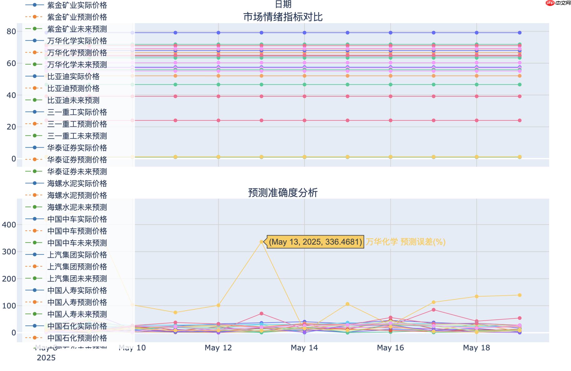
subplot_titles=( "价格预测对比", "市场情绪指标对比", "预测准确度分析"
)
)
# 为每只股票添加价格预测线
for ticker in combined_data['Ticker'].unique():
stock_data = combined_data[combined_data['Ticker'] == ticker]
name = stock_data['Name'].iloc[0]
# 实际价格线
fig.add_trace(
go.Scatter(
x=stock_data['Date'],
y=stock_data['Actual'],
name=f"{name}实际价格",
line=dict(color=self.colors['actual'], width=1)
),
row=1, col=1
)
# 预测价格线
fig.add_trace(
go.Scatter(
x=stock_data['Date'],
y=stock_data['Predicted'],
name=f"{name}预测价格",
line=dict(color=self.colors['predicted'], width=1, dash='dot')
),
row=1, col=1
)
# 未来预测线
future_data = stock_data[stock_data['Future_Predicted'].notna()] if not future_data.empty:
fig.add_trace(
go.Scatter(
x=future_data['Date'],
y=future_data['Future_Predicted'],
name=f"{name}未来预测",
line=dict(color=self.colors['future'], width=1, dash='dash')
),
row=1, col=1
)
# 添加市场情绪指标对比
for ticker in combined_data['Ticker'].unique():
stock_data = combined_data[combined_data['Ticker'] == ticker]
name = stock_data['Name'].iloc[0]
# MFI指标线
fig.add_trace(
go.Scatter(
x=stock_data['Date'],
y=stock_data['MFI'],
name=f"{name} MFI",
line=dict(width=1)
),
row=2, col=1
)
# 趋势强度线
fig.add_trace(
go.Scatter(
x=stock_data['Date'],
y=stock_data['Trend_Strength'],
name=f"{name} 趋势强度",
line=dict(width=1)
),
row=2, col=1
)
# 添加预测准确度分析
for ticker in combined_data['Ticker'].unique():
stock_data = combined_data[combined_data['Ticker'] == ticker]
name = stock_data['Name'].iloc[0]
# 计算预测误差
error = np.abs(stock_data['Predicted'] - stock_data['Actual']) / stock_data['Actual'] * 100
fig.add_trace(
go.Scatter(
x=stock_data['Date'],
y=error,
name=f"{name} 预测误差(%)",
line=dict(width=1)
),
row=3, col=1
)
# 更新布局
fig.update_layout(
title=title,
xaxis_title="日期",
height=1200, # 图表高度
showlegend=True,
legend=dict(
yanchor="top",
y=0.99,
xanchor="left",
x=0.01,
bgcolor="rgba(255, 255, 255, 0.8)"
)
)
# 添加网格线
fig.update_xaxes(showgrid=True, gridwidth=1, gridcolor='LightGray')
fig.update_yaxes(showgrid=True, gridwidth=1, gridcolor='LightGray')
# 保存为HTML文件
html_file = f"{title.replace(' ', '_')}.html"
fig.write_html(html_file, include_plotlyjs=True, full_html=True)
return html_filedef plot_multiple_predictions(self, results, title="多股票预测分析"):
"""
绘制多只股票的预测对比图
参数详解:
results: List[Dict], 包含每只股票预测结果的列表
title: str, 图表标题
返回:
plotly.graph_objects.Figure: 生成的图表对象
"""
fig = go.Figure() # 按预测涨跌幅排序
sorted_results = sorted(
results,
key=lambda x: x['future_change'] if x['future_change'] is not None else -float('inf'),
reverse=True
) # 添加每只股票的预测涨跌幅柱状图
fig.add_trace(go.Bar(
x=[f"{r['name']}({r['ticker']})" for r in sorted_results],
y=[r['future_change'] for r in sorted_results],
marker_color=[self.colors['trend_up'] if c > 0 else self.colors['trend_down']
for c in [r['future_change'] for r in sorted_results]],
text=[f"{c:.2f}%" for c in [r['future_change'] for r in sorted_results]],
textposition='auto',
)) # 更新布局
fig.update_layout(
title=title,
xaxis_title="股票",
yaxis_title="预测涨跌幅(%)",
template='plotly_white', # 使用白色主题
height=600,
showlegend=False,
xaxis_tickangle=-45, # 标签倾斜角度
plot_bgcolor='white',
paper_bgcolor='white',
margin=dict(l=50, r=50, t=50, b=50) # 边距设置
) return figdef plot_prediction_accuracy(self, results, title="预测准确度分析"):
"""
绘制预测准确度分析图
参数详解:
results: List[Dict], 包含每只股票预测结果的列表
title: str, 图表标题
返回:
plotly.graph_objects.Figure: 生成的图表对象
"""
# 创建子图布局
fig = make_subplots(
rows=1, cols=2,
subplot_titles=("RMSE分布", "预测准确度与涨跌幅关系")
) # RMSE分布箱线图
rmse_values = [r['metrics']['rmse'] for r in results]
fig.add_trace(
go.Box(y=rmse_values, name="RMSE分布"),
row=1, col=1
) # RMSE vs 涨跌幅散点图
fig.add_trace(
go.Scatter(
x=[r['future_change'] for r in results],
y=[r['metrics']['rmse'] for r in results],
mode='markers+text',
text=[r['name'] for r in results],
textposition="top center",
marker=dict(
size=10,
color=[r['future_change'] for r in results],
colorscale='RdYlBu', # 红黄蓝色阶
showscale=True
),
name="股票分布"
),
row=1, col=2
) # 更新布局
fig.update_layout(
title_text=title,
height=500,
template='plotly_white',
showlegend=False
) # 更新坐标轴
fig.update_xaxes(title_text="预测涨跌幅(%)", row=1, col=2)
fig.update_yaxes(title_text="RMSE", row=1, col=1)
fig.update_yaxes(title_text="RMSE", row=1, col=2) return figdef create_analysis_dashboard(self, stock_data, predictions, results, future_predictions=None):
"""
创建完整的分析仪表板
参数详解:
stock_data: pd.DataFrame, 原始股票数据
predictions: np.ndarray, 模型预测结果
results: List[Dict], 预测结果列表
future_predictions: np.ndarray, 未来价格预测
返回:
Dict: 包含所有图表的字典
"""
# 创建各个图表
stock_fig = self.plot_stock_prediction(stock_data, predictions, future_predictions)
multi_pred_fig = self.plot_multiple_predictions(results)
accuracy_fig = self.plot_prediction_accuracy(results)
# 返回所有图表
return { 'stock_prediction': stock_fig, 'multiple_predictions': multi_pred_fig, 'prediction_accuracy': accuracy_fig
}以上就是【新手入门】0基础学习用AI模型进行预测(以A股股票场景为例、基于Paddle)的详细内容,更多请关注php中文网其它相关文章!

每个人都需要一台速度更快、更稳定的 PC。随着时间的推移,垃圾文件、旧注册表数据和不必要的后台进程会占用资源并降低性能。幸运的是,许多工具可以让 Windows 保持平稳运行。

Copyright 2014-2025 https://www.php.cn/ All Rights Reserved | php.cn | 湘ICP备2023035733号


 190
190