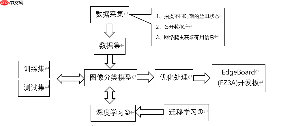
本项目针对我国沿海圈围晒盐依赖人工巡视的现状,利用飞桨平台的图像分类技术,通过相机定时拍照上传图像,实现盐田状态智能识别。为盐田编号,实时观测卤水水量、结晶程度等,判断操作时机,估测盐品质与产量。经数据采集、模型构建训练,可辅助管理人员高效管理盐田,节省人力成本,提升出盐效率,具有良好应用前景。
☞☞☞AI 智能聊天, 问答助手, AI 智能搜索, 免费无限量使用 DeepSeek R1 模型☜☜☜

通过飞桨开源深度学习平图像分类技术将检测到的信息实时传输给小程序。实现了由机器自动识别与分类去代替人工巡视。
相机每隔30分钟拍照上传图像数据至系统,系统自动识别判断盐田需要进行何种操作。
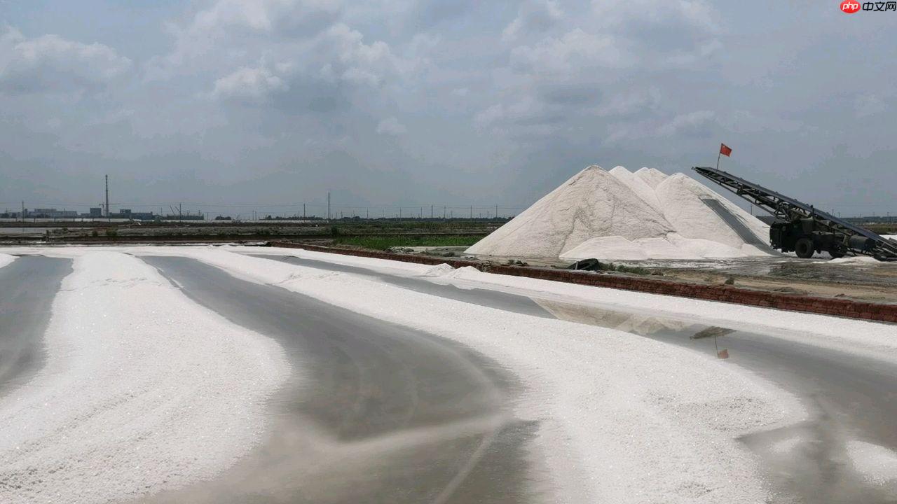
我国沿海地区,有很多盐场,通过圈围海水或高盐度井水的方式,在太阳下暴晒,使水分蒸发掉,逐渐结晶形成固态的盐。
目前我国圈围式晒盐还采取较为传统的人工巡视方式,极大的耗费人力资源,盐场巡视晒盐尚未涉及到人工智能领域,目前还没有相应的产品和服务。
a.为每个盐田编号并利用图像识别技术,实时观测盐田中卤水的水量和卤水的结晶程度,精确的处理数据并将数据传输给管理人员。我们可以通过设备实时观测盐田中卤水的高度、水量和盐的结晶程度,通过对这些数据的整合,分析出什么时候该加水,什么时候该搂盐,什么时候可以捞盐归坨,还可以计算出盐的产量,判断盐的品质,大大的提高了出盐效率。
b.通过图像识别,能大面积初步对盐的品质和产量进行估测。采用智能化管理每个管理员都可以管理更多的盐田,经济可靠、节省人工成本、方便用户使用。
由于目前我国沿海地区大部分还是采用圈围晒盐的方式,通过纯人为对盐田进行巡视管理既费时又费力,还需要大量工人。一般每十个盐田就需要一个工人管理,工人要亲自检测卤水的浓度、水量多少和卤水的结晶情况,沿海地区盐田分布广泛,采用本产品智能化管理可以大量节省人工、提高工作效率。
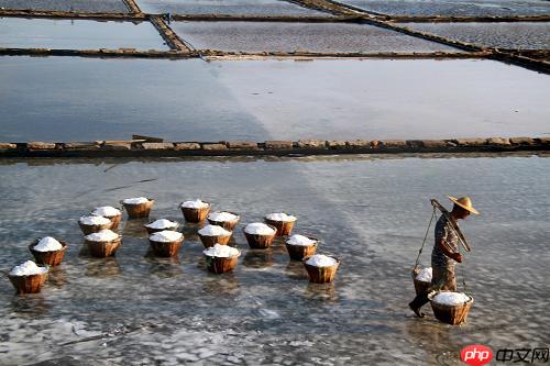
盐场工人正在搂盐、收盐


a.采集数据阶段,采用飞桨平台建立项目创建一个数据集,对盐田不同阶段、不同光照环境下的状态进行大量拍照取证,通过对相似的数据保留,对个别特殊情况建立特殊数据集。采用不同的图像分类模型,将数据集放入模型中通过飞桨平台提供的算力模拟与实际结果进行比对,最后确立准确度较高的模型进行应用。
b.确立采用的模型后,进行优化算法处理,对梯度下降使用方式、参数更新方式、步长等进行设置。定义输出日志,打印训练过程中得到的模型在验证集上的精确度和在训练集上的精确度,获知模型是否过(欠)拟合。在后期数据不断更新中也可以对计算机进行训练与测试,最终获得的模型参数的保存进微型计算机中。
c.数据处理:
本项目目前数据较为缺乏,采用迁移学习可以很好地利用相关领域有标定的数据完成数据的标定。
深度学习系统是确立好模型后,导入数据和预处理,处理数据集的数据,使之适合模型使用,对几种经典的模型,例如AlexNet,VGG,GoogLeNet /Inception, ResNet,进行比较筛选,把所有的代码交给平台运行,平台自动训练模型,最后选出合适的模型。
验初始阶段,我们用自行采集的方式获取初始数据,通过将数据经整理后存入数据集。
队员们在收集数据
本项目采集完数据后我们进行数据的清洗工作, 数据清洗是整合数据后所需要进行的数据预处理工作。在这一步,我们通过检查数据表和目标变量的格式、删除所有值都缺失的变量、删除低方差的变量、将唯一值比例大于一定阈值的变量二值化、对缺失值比例大于一定阈值的变量进行二值化处理、合并类别个数超过一定数目的变量类别、删除重复的观察样本、处理异常值、处理缺失值等操作将脏数据清理为相对比较规整的数据。对于图像分类任务,我们只要将对应的图片是哪个类别划分好即可。对于检测任务和分割任务,目前比较流行的数据标注工具是labelimg、labelme,分别用于检测任务与分割任务的标注。
采用预设的数据变换规则,在已有数据的基础上进行数据的扩增,包含单样本数据增强和多样本数据增强,其中单样本又包括几何操作类,颜色变换类。围绕着单样本数据本身进行数据增强处理。
#解压上传到AI Studio的压缩包!ls /home/aistudio/dataimport osimport zipfile
os.chdir('/home/aistudio/data/data100510')
extracting = zipfile.ZipFile('salt pan.zip')
extracting.extractall()data100510
#!/usr/bin/env python# coding: utf-8#对数据集生成固定格式的列表,格式为:图片的路径 <Tab> 图片类别的标签import jsonimport osdef create_data_list(data_root_path):
    with open(data_root_path + "test.list", 'w') as f:        pass
    with open(data_root_path + "train.list", 'w') as f:        pass
    # 所有类别的信息
    class_detail = []    # 获取所有类别
    class_dirs = os.listdir(data_root_path)    # 类别标签
    class_label = 0
    # 获取总类别的名称
    father_paths = data_root_path.split('/')    while True:        if father_paths[len(father_paths) - 1] == '':            del father_paths[len(father_paths) - 1]        else:            break
    father_path = father_paths[len(father_paths) - 1]

    all_class_images = 0
    other_file = 0
    # 读取每个类别
    for class_dir in class_dirs:        if class_dir == 'test.list' or class_dir == "train.list" or class_dir == 'readme.json':
            other_file += 1
            continue
        print('正在读取类别:%s' % class_dir)        # 每个类别的信息
        class_detail_list = {}
        test_sum = 0
        trainer_sum = 0
        # 统计每个类别有多少张图片
        class_sum = 0
        # 获取类别路径
        path = data_root_path + "/" + class_dir        # 获取所有图片
        img_paths = os.listdir(path)        for img_path in img_paths:            # 每张图片的路径
            name_path = class_dir + '/' + img_path            # 如果不存在这个文件夹,就创建
            if not os.path.exists(data_root_path):
                os.makedirs(data_root_path)            # 划分训练集和测试集,各个类别中每隔十张选取一张作为测试集,并将数据集生成固定格式列表。
            if class_sum % 10 == 0:
                test_sum += 1
                with open(data_root_path + "test.list", 'a') as f:
                    f.write(name_path + "\t%d" % class_label + "\n")            else:
                trainer_sum += 1
                with open(data_root_path + "train.list", 'a') as f:
                    f.write(name_path + "\t%d" % class_label + "\n")
            class_sum += 1
            all_class_images += 1
        # 说明的json文件的class_detail数据
        class_detail_list['class_name'] = class_dir
        class_detail_list['class_label'] = class_label
        class_detail_list['class_test_images'] = test_sum
        class_detail_list['class_trainer_images'] = trainer_sum
        class_detail.append(class_detail_list)
        class_label += 1
    # 获取类别数量
    all_class_sum = len(class_dirs) - other_file    # 说明的json文件信息
    readjson = {}
    readjson['all_class_name'] = father_path
    readjson['all_class_sum'] = all_class_sum
    readjson['all_class_images'] = all_class_images
    readjson['class_detail'] = class_detail
    jsons = json.dumps(readjson, sort_keys=True, indent=4, separators=(',', ': '))    with open(data_root_path + "readme.json", 'w') as f:
f.write(jsons) print('图像列表已生成')#生成图像的列表if __name__ == '__main__': # 把生产的数据列表都放在自己的总类别文件夹中
data_root_path = "salt pan/"
create_data_list(data_root_path)正在读取类别:Salt5_level13 正在读取类别:Salt5_level14 正在读取类别:Salt3_level12 正在读取类别:Salt7_level16 正在读取类别:Salt5_level11 正在读取类别:Salt4_level14 正在读取类别:Salt5_level12 正在读取类别:Salt4_level12 正在读取类别:Salt5_level15 正在读取类别:Salt5_level16 正在读取类别:Salt7_level12 图像列表已生成
采用飞桨平台建立项目创建一个数据集,对盐田不同阶段、不同光照环境下的状态进行大量拍照取证,通过对相似的数据保留,对个别特殊情况建立特殊数据集。采用不同的图像分类模型,将数据集放入模型中通过飞桨平台提供的算力模拟与实际结果进行比对,最后确立准确度较高的模型进行应用。为此,本项目构建了首个盐田不同时期状态数据集,并计划在与版权所有方完成全部细节沟通后进行开源。
我们的盐田不同时期状态数据集主要来自队员的采集
#架构模型时需要用到的组件。#包括BN层、常规卷积层、xavier初始化方法#以及改进后的inception结构(salt-inception)和深度可分离卷积结构import paddle.fluid as fluidimport numpy as npimport timeimport mathimport paddleimport paddle.fluid as fluidimport codecsimport loggingfrom paddle.fluid.initializer import MSRAfrom paddle.fluid.initializer import Uniformfrom paddle.fluid.param_attr import ParamAttrfrom PIL import Imagefrom PIL import ImageEnhanceimport osimport randomfrom multiprocessing import cpu_countimport numpy as npimport paddlefrom PIL import Image


#BN层def conv_bn_layer(input, filter_size, num_filters, stride,
                  padding, channels=None, num_groups=1, act='relu', use_cudnn=True):
    conv = fluid.layers.conv2d(input=input,
                               num_filters=num_filters,
                               filter_size=filter_size,
                               stride=stride,
                               padding=padding,
                               groups=num_groups,
                               act=None,
                               use_cudnn=use_cudnn,
                               bias_attr=False)    return fluid.layers.batch_norm(input=conv, act=act)#常规卷积层def conv_layer(
           input,
           num_filters,
           filter_size,
           stride=1,
           groups=1,
           act=None,
           name=None):
    channels = input.shape[1]
    stdv = (3.0 / (filter_size**2 * channels))**0.5
    param_attr = ParamAttr(
        initializer=fluid.initializer.Uniform(-stdv, stdv),
        name=name + "_weights")
    conv = fluid.layers.conv2d(        input=input,
        num_filters=num_filters,
        filter_size=filter_size,
        stride=stride,
        padding=(filter_size - 1) // 2,
        groups=groups,
        act=act,
        param_attr=param_attr,
        bias_attr=False,
        name=name)    return convdef xavier(self, channels, filter_size, name):
    stdv = (3.0 / (filter_size**2 * channels))**0.5
    param_attr = ParamAttr(
        initializer=fluid.initializer.Uniform(-stdv, stdv),
        name=name + "_weights")
    return param_attr#改进后的inception结构(salt-inception)def inception(
          input,
          channels,
          filter1,
          filter3R,
          filter3,
          filter5R,
          filter5,
          filter7R,
          filter7,
          proj,
          name=None):
    conv1 = conv_layer(        input=input,
        num_filters=filter1,
        filter_size=1,
        stride=1,
        act=None,
        name="inception_" + name + "_1x1")
    #由一个1*1卷积层和一个3*3卷积层组成salt-inception的支路
    conv3r = conv_layer(        input=input,
        num_filters=filter3R,
        filter_size=1,
        stride=1,
        act=None,
        name="inception_" + name + "_3x3_reduce")
    conv3 = conv_layer(        input=conv3r,
        num_filters=filter3,
        filter_size=3,
        stride=1,
        act=None,
        name="inception_" + name + "_3x3")
    #由一个1*1卷积层和2个3*3卷积层组成salt-inception的支路,由2个3*3卷积层代替5*5卷积层
    conv5r = conv_layer(        input=input,
        num_filters=filter5R,
        filter_size=1,
        stride=1,
        act=None,
        name="inception_" + name + "_5x5_reduce")
    conv5 = conv_layer(        input=conv5r,
        num_filters=filter5R,
        filter_size=3,
        stride=1,
        act=None,
        name="inception_" + name + "_5x5")
    conv5 = conv_layer(        input=conv5,
        num_filters=filter5,
        filter_size=3,
        stride=1,
        act=None,
        name="inception_" + name + "_5x5_2")    #由一个1*1卷积层和3个3*3卷积层组成salt-inception的支路,由3个3*3卷积层代替7*7卷积层
    conv7r = conv_layer(        input=input,
        num_filters=filter7R,
        filter_size=1,
        stride=1,
        act=None,
        name="inception_" + name + "_7x7_reduce")
    conv7 = conv_layer(        input=conv7r,
        num_filters=filter7R,
        filter_size=3,
        stride=1,
        act=None,
        name="inception_" + name + "_7x7")
    conv7 = conv_layer(        input=conv7,
        num_filters=filter7R,
        filter_size=3,
        stride=1,
        act=None,
        name="inception_" + name + "_7x7_2")
    conv7 = conv_layer(        input=conv7,
        num_filters=filter7,
        filter_size=3,
        stride=1,
        act=None,
        name="inception_" + name + "_7x7_3")

    pool = fluid.layers.pool2d(        input=input,
        pool_size=3,
        pool_stride=1,
        pool_padding=1,
        pool_type='max')
    convprj = fluid.layers.conv2d(        input=pool,
        filter_size=1,
        num_filters=proj,
        stride=1,
        padding=0,
        name="inception_" + name + "_3x3_proj",
        param_attr=ParamAttr(
            name="inception_" + name + "_3x3_proj_weights"),
        bias_attr=False)
    cat = fluid.layers.concat(input=[conv1, conv3, conv5, conv7, convprj], axis=1)
    cat = fluid.layers.relu(cat)    return cat#深度可分离卷积def depthwise_separable(input, num_filters1, num_filters2, num_groups, stride, scale):
    depthwise_conv = conv_bn_layer(input=input,
                                   filter_size=3,
                                   num_filters=int(num_filters1 * scale),
                                   stride=stride,
                                   padding=1,
                                   num_groups=int(num_groups * scale),
                                   use_cudnn=False)

    pointwise_conv = conv_bn_layer(input=depthwise_conv,
                                   filter_size=1,
                                   num_filters=int(num_filters2 * scale),
                                   stride=1,
padding=0) return pointwise_conv#salt-ConvNet卷积神经网络的结构def net(input, class_dim, scale=1.0):
# 224x224
input = conv_bn_layer(input=input,
filter_size=3,
channels=3,
num_filters=int(32 * scale),
stride=2,
padding=1)
# 112x112
input = depthwise_separable(input=input,
num_filters1=32,
num_filters2=64,
num_groups=32,
stride=1,
scale=scale)
input = depthwise_separable(input=input,
num_filters1=64,
num_filters2=128,
num_groups=64,
stride=2,
scale=scale)
# 56x56
input = depthwise_separable(input=input,
num_filters1=128,
num_filters2=128,
num_groups=128,
stride=1,
scale=scale) input = depthwise_separable(input=input,
num_filters1=128,
num_filters2=256,
num_groups=128,
stride=2,
scale=scale)
# 28x28
input = depthwise_separable(input=input,
num_filters1=256,
num_filters2=256,
num_groups=256,
stride=1,
scale=scale) input = depthwise_separable(input=input,
num_filters1=256,
num_filters2=512,
num_groups=256,
stride=2,
scale=scale)
# 14x14
input = inception(input, 480, 192, 96, 208, 16, 24, 16, 24,64, "input")
input1 = inception(input, 512, 160, 112, 224, 24, 32, 24, 32, 64, "input1")
input1 = paddle.fluid.layers.concat(input=[input,input1], axis=1)
input2 = inception(input1, 512, 128, 128, 256, 24, 32, 24, 32, 64, "input2")
input2 = paddle.fluid.layers.concat(input=[input,input1,input2], axis=1)
input3 = inception(input2, 512, 128, 128, 256, 24, 32, 24, 32, 64, "input3")
input3 = paddle.fluid.layers.concat(input=[input,input1,input2,input3], axis=1)
input = depthwise_separable(input=input3,
num_filters1=512,
num_filters2=1024,
num_groups=512,
stride=2,
scale=scale)
# 7x7
input = depthwise_separable(input=input,
num_filters1=1024,
num_filters2=1024,
num_groups=1024,
stride=1,
scale=scale)
feature = fluid.layers.pool2d(input=input,
pool_size=0,
pool_stride=1,
pool_type='avg',
global_pooling=True)
net = fluid.layers.fc(input=feature,
size=class_dim,
act='softmax') return net# 训练图片的预处理import random
from PIL import Imagedef train_mapper(sample):
img_path, label, crop_size, resize_size = sample
img = Image.open(img_path) # 统一图片大小
img = img.resize((resize_size, resize_size), Image.ANTIALIAS) # 随机水平翻转
r1 = random.random() if r1 > 0.5:
img = img.transpose(Image.FLIP_LEFT_RIGHT) # 随机垂直翻转
r2 = random.random() if r2 > 0.5:
img = img.transpose(Image.FLIP_TOP_BOTTOM) # 随机角度翻转
r3 = random.randint(-3, 3)
img = img.rotate(r3, expand=False) # 随机裁剪
r4 = random.randint(0, int(resize_size - crop_size))
r5 = random.randint(0, int(resize_size - crop_size))
box = (r4, r5, r4 + crop_size, r5 + crop_size)
img = img.crop(box) # 把图片转换成numpy值
img = np.array(img).astype(np.float32) # 转换成CHW
img = img.transpose((2, 0, 1)) # 转换成BGR
img = img[(2, 1, 0), :, :] / 255.0
return img, int(label)# 获取训练的readerdef train_r(train_list_path, crop_size, resize_size):
father_path = os.path.dirname(train_list_path) def reader():
with open(train_list_path, 'r') as f:
lines = f.readlines() # 打乱图像列表
np.random.shuffle(lines) # 开始获取每张图像和标签
for line in lines:
img, label = line.split('\t')
img = os.path.join(father_path, img) yield img, label, crop_size, resize_size return paddle.reader.xmap_readers(train_mapper, reader, cpu_count(), 102400)# 测试图片的预处理def test_mapper(sample):
img, label, crop_size = sample
img = Image.open(img) # 统一图像大小
img = img.resize((crop_size, crop_size), Image.ANTIALIAS) # 转换成numpy值
img = np.array(img).astype(np.float32) # 转换成CHW
img = img.transpose((2, 0, 1)) # 转换成BGR
img = img[(2, 1, 0), :, :] / 255.0
return img, int(label)# 测试的图片readerdef test_r(test_list_path, crop_size):
father_path = os.path.dirname(test_list_path) def reader():
with open(test_list_path, 'r') as f:
lines = f.readlines() for line in lines:
img, label = line.split('\t')
img = os.path.join(father_path, img) yield img, label, crop_size return paddle.reader.xmap_readers(test_mapper, reader, cpu_count(), 1024)#进行模型的训练import osimport shutilimport paddle as paddleimport paddle.fluid as fluidfrom multiprocessing import cpu_countimport numpy as npimport os
crop_size = 224resize_size = 250# 获取划分好的训练集和数据集,注意传入的.list文件的路径是否正确try:
os.chdir('/home/aistudio/data/data100510')except: passtrain_reader = paddle.batch(reader=train_r('salt pan/train.list', crop_size, resize_size), batch_size=32)
test_reader = paddle.batch(reader=test_r('salt pan/test.list', crop_size), batch_size=32)# 定义网络def vgg_test_net(image, type_size):
def conv_block(ipt, num_filter, groups, dropouts):
return fluid.nets.img_conv_group( input=ipt, # 具有[N,C,H,W]格式的输入图像
pool_size=2,
pool_stride=2,
conv_num_filter=[num_filter] * groups, # 过滤器个数
conv_filter_size=3, # 过滤器大小
conv_act='relu',
conv_with_batchnorm=True, # 表示在 Conv2d Layer 之后是否使用 BatchNorm
conv_batchnorm_drop_rate=dropouts,# 表示 BatchNorm 之后的 Dropout Layer 的丢弃概率
pool_type='max') # 最大池化
conv1 = conv_block(image, 64, 2, [0.0, 0])
conv2 = conv_block(conv1, 128, 2, [0.0, 0])
conv3 = conv_block(conv2, 256, 3, [0.0, 0.0, 0])
conv4 = conv_block(conv3, 512, 3, [0.0, 0.0, 0])
conv5 = conv_block(conv4, 512, 3, [0.0, 0.0, 0])
drop = fluid.layers.dropout(x=conv2, dropout_prob=0.5)
fc1 = fluid.layers.fc(input=drop, size=512, act=None)
bn = fluid.layers.batch_norm(input=fc1, act='relu')
drop2 = fluid.layers.dropout(x=bn, dropout_prob=0.0)
fc2 = fluid.layers.fc(input=drop2, size=512, act=None) # predict = fluid.layers.fc(input=fc1, size=type_size, act='softmax')
predict = fluid.layers.fc(input=fc1, size=type_size) return predict# 定义输入层paddle.enable_static()
image = fluid.layers.data(name='image', shape=[3, crop_size, crop_size], dtype='float32')
label = fluid.layers.data(name='label', shape=[1], dtype='int64')# 调用构建好的网络模型salt-ConvNet,并对11种盐田进行分类。predict = net(image, 11)#疑似出错!!!!!!!!!!!# 获取损失函数(交叉熵函数)和准确率函数cost = fluid.layers.cross_entropy(input=predict, label=label)
avg_cost = fluid.layers.mean(cost)
acc = fluid.layers.accuracy(input=predict, label=label)# 获取训练和测试程序test_program = fluid.default_main_program().clone(for_test=True)# 定义优化方法为Adamoptimizer = fluid.optimizer.AdamOptimizer(learning_rate=1e-3,
regularization=fluid.regularizer.L2DecayRegularizer(1e-4))
opts = optimizer.minimize(avg_cost)# 定义一个使用GPU的执行器place = fluid.CUDAPlace(0)# place = fluid.CPUPlace()exe = fluid.Executor(place)# 进行参数初始化exe.run(fluid.default_startup_program())# 定义输入数据维度feeder = fluid.DataFeeder(place=place, feed_list=[image, label])确立采用的模型后,进行优化算法处理,对梯度下降使用方式、参数更新方式、步长等进行设置。定义输出日志,打印训练过程中得到的模型在验证集上的精确度和在训练集上的精确度,获知模型是否过(欠)拟合。在后期数据不断更新中也可以对计算机进行训练与测试,最终获得的模型参数的保存进微型计算机中达到了良好的效果。
算法运行图
# 训练30轮for pass_id in range(30):    # 进行训练
    for batch_id, data in enumerate(train_reader()):
        train_cost, train_acc = exe.run(program=fluid.default_main_program(),
                                        feed=feeder.feed(data),
                                        fetch_list=[avg_cost, acc])        # 每100个batch打印一次信息
        if batch_id % 10 == 0:            print('Pass:%d, Batch:%d, Cost:%0.5f, Accuracy:%0.5f' %
                  (pass_id, batch_id, train_cost[0], train_acc[0]))    # 进行测试
    test_accs = []
    test_costs = []    for batch_id, data in enumerate(test_reader()):
        test_cost, test_acc = exe.run(program=test_program,
                                      feed=feeder.feed(data),
                                      fetch_list=[avg_cost, acc])
        test_accs.append(test_acc[0])
        test_costs.append(test_cost[0])    # 求测试结果的平均值
    test_cost = (sum(test_costs) / len(test_costs))
    test_acc = (sum(test_accs) / len(test_accs))    print('Test:%d, Cost:%0.5f, Accuracy:%0.5f' % (pass_id, test_cost, test_acc))
    # 保存预测模型
    save_path = 'infer_model/'
    # 删除旧的模型文件
    shutil.rmtree(save_path, ignore_errors=True)    # 创建保持模型文件目录
    os.makedirs(save_path)    # 保存预测模型
fluid.io.save_inference_model(save_path, feeded_var_names=[image.name], target_vars=[predict], executor=exe)Pass:0, Batch:0, Cost:2.46918, Accuracy:0.15625
import cv2from PIL import Imageimport random
# data = cv2.imread("/home/aistudio/data/data100510/salt pan/Salt5_level16/8 (38).jpg")img = Image.open("/home/aistudio/data/data100510/salt pan/Salt5_level16/8 (38).jpg")print(img)# 统一图片大小img = img.resize((resize_size, resize_size), Image.ANTIALIAS)# 随机水平翻转r1 = random.random()if r1 > 0.5:
    img = img.transpose(Image.FLIP_LEFT_RIGHT)# 随机垂直翻转r2 = random.random()if r2 > 0.5:
    img = img.transpose(Image.FLIP_TOP_BOTTOM)# 随机角度翻转r3 = random.randint(-3, 3)
img = img.rotate(r3, expand=False)# 随机裁剪r4 = random.randint(0, int(resize_size - crop_size))
r5 = random.randint(0, int(resize_size - crop_size))
box = (r4, r5, r4 + crop_size, r5 + crop_size)
img = img.crop(box)# 把图片转换成numpy值img = np.array(img).astype(np.float32) # 转换成CHWimg = img.transpose((2, 0, 1)) # 转换成BGRimg = img[(2, 1, 0), :, :] / 255.0print(img)<PIL.JpegImagePlugin.JpegImageFile image mode=RGB size=3648x2736 at 0x7FEF31325510> [[[0.6431373 0.5647059 0.54901963 ... 0.7490196 0.7411765 0.7529412 ] [0.60784316 0.5568628 0.61960787 ... 0.7490196 0.7294118 0.74509805] [0.5882353 0.61960787 0.63529414 ... 0.7411765 0.7254902 0.7529412 ] ... [0.68235296 0.6901961 0.68235296 ... 0.7490196 0.7294118 0.70980394] [0.6784314 0.68235296 0.68235296 ... 0.7647059 0.7529412 0.73333335] [0. 0. 0. ... 0.76862746 0.7607843 0.74509805]] [[0.7058824 0.627451 0.6117647 ... 0.70980394 0.7058824 0.7137255 ] [0.67058825 0.61960787 0.68235296 ... 0.7058824 0.69803923 0.7137255 ] [0.6509804 0.68235296 0.69803923 ... 0.7019608 0.69411767 0.7254902 ] ... [0.70980394 0.7137255 0.7058824 ... 0.7058824 0.6862745 0.6666667 ] [0.7058824 0.70980394 0.7058824 ... 0.72156864 0.70980394 0.6901961 ] [0. 0. 0. ... 0.7294118 0.7176471 0.7019608 ]] [[0.77254903 0.69411767 0.6784314 ... 0.7137255 0.7137255 0.7176471 ] [0.7372549 0.6862745 0.7490196 ... 0.7137255 0.7019608 0.7176471 ] [0.7176471 0.7490196 0.7647059 ... 0.7058824 0.7019608 0.73333335] ... [0.7529412 0.75686276 0.7490196 ... 0.7137255 0.69411767 0.6745098 ] [0.7490196 0.7529412 0.7490196 ... 0.7294118 0.7176471 0.69803923] [0. 0. 0. ... 0.7372549 0.7254902 0.70980394]]]
加载好训练的模型,对某一特定输入的盐田图片进行测试
import paddle.fluid as fluidfrom PIL import Imageimport numpy as np# 创建执行器place = fluid.CPUPlace()
exe = fluid.Executor(place)
exe.run(fluid.default_startup_program())# 保存预测模型路径save_path = 'infer_model/'# 从模型中获取预测程序、输入数据名称列表、分类器[infer_program, feeded_var_names, target_var] = fluid.io.load_inference_model(dirname=save_path, executor=exe)# 预处理图片def load_image(file):
    img = Image.open(file)    # 统一图像大小
    img = img.resize((224, 224), Image.ANTIALIAS)    # 转换成numpy值
    img = np.array(img).astype(np.float32)    # 转换成CHW
    img = img.transpose((2, 0, 1))    # 转换成BGR
    img = img[(2, 1, 0), :, :] / 255.0
    img = np.expand_dims(img, axis=0)    return img# 获取图片数据,可以更改imgpath的值,实现对不同的图片进行预测。imgpath = "/home/aistudio/salt3_level12.jpg"img = load_image(imgpath)# 执行预测result = exe.run(program=infer_program,
                 feed={feeded_var_names[0]: img},
                 fetch_list=target_var)# 显示图片并输出结果最大的labellab = np.argsort(result)[0][0][-1]

names = ['Salt3_level12', 'Salt4_level12', 'Salt4_level14','Salt5_level11', 'Salt5_level12','Salt5_level13','Salt5_level14','Salt5_level15','Salt5_level16','Salt7_level12','Salt7_level16']print('图片路径为:%s, 预测结果标签为:%d, 预测结果为:%s, 概率为:%f' % (imgpath, lab, names[lab], result[0][0][lab]))图片路径为:/home/aistudio/salt3_level12.jpg, 预测结果标签为:10, 预测结果为:Salt7_level16, 概率为:0.861619
视频链接: https://www.bilibili.com/video/BV1q3411z7hr?share_source=copy_web/
我国海域广大,海水盐度高,海岸线漫长,滩地平坦,晴日多光照强,晒盐条件与产盐的品质都十分优越。并且我国海盐产量巨大,年产量2000万吨,为世界第一大海盐产量国。目前海盐产量仍满足不了供应需求,由于国内烧碱和纯碱等基础化工原料产量不断增加,对海盐的需求也不断提升,预计未来几年内每年的缺口在1000万吨左右。所以,在晒盐技术创新方面有着巨大的市场前景与实用价值。
以上就是【飞桨领航团AI达人创造营】基于EdgeBoard部署的圈围晒盐的智能辅助系统的详细内容,更多请关注php中文网其它相关文章!

每个人都需要一台速度更快、更稳定的 PC。随着时间的推移,垃圾文件、旧注册表数据和不必要的后台进程会占用资源并降低性能。幸运的是,许多工具可以让 Windows 保持平稳运行。

Copyright 2014-2025 https://www.php.cn/ All Rights Reserved | php.cn | 湘ICP备2023035733号


 172
172